Avalekander Week 7
Purpose
The purpose of this week is to analyze the regulatory networks and determine a future in silico experiment to better represent the data.
Methods
Analyzing Results of First Model Run
Here is what was considered when results of the model were analyzed.
- Determine the LSE on the "optimization_diagnostics" worksheet of your output workbook.
- Compute the LSE:LSEmin ratio by looking at the values given on the "optimization_diagnostics" worksheet.
- Then in class the LSE:minLSE ratios were compared for the ten models run by everyone in the class.
- Look at the individual fits for each of the genes in the model and decide which genes are modeled well and which are not modeled well.
- Additionally, look at the individual expression plots to see if the line that represents the simulated model data is a good fit to the individual data points.
- Upload your output Excel spreadsheet to GRNsight. Use the dropdown menu on the left to choose the data you will display on the nodes (boxes). Compare the actual data for a strain with the simulated data from the same strain. If the model fits the data well, the color heatmap superimposed on the node will match top and bottom. If the fit is less good, the colors will not match.
- Answer the following:
- What explains the goodness of fit to the model?
- How many arrows are incoming to the node?
- What is the ANOVA Benjamini & Hochberg corrected p value for the gene?
- Is the gene changing its expression a lot or is the log2 fold change mostly near zero?
- What explains the goodness of fit to the model?
- Make bar charts for the b and P parameters.
- Is there something about these parameters that explains the goodness of fit for the individual genes?
Tweaking the Model and Analyzing the Results
An additional in silico experiment will be performed with the model. Some ideas are:
- For our initial runs, we estimated all three parameters w, P, and b.
- How do the modeling results change if P is instead fixed and w and b are estimated?
- How do the modeling results change if b is fixed and w and P are estimated?
- How do the modeling results change if P and b are fixed, and only w is estimated?
- For our initial runs, we included all three microarray datasets, wt, Δgln3, and Δhap4.
- What happens to the results if we base the estimation on just two strains (wt + one deletion strain)?
- What happens to the results if we base the estimation on just the wt strain data?
- When viewing the modeling results in GRNsight, you may determine that one or more genes in the network does not appear to be doing much.
- What happens to the modeling results if you delete this gene from the network and re-run the model (remember you will have to delete references to this gene in all worksheets of the input file).
- You also might think that a particular edge (regulatory relationship) is not needed. What happens if you delete that edge?
- What happens if you include the t90 and t120 expression data?
Results
GRNsight Gene Regulatory Network
- GRNsight regulatory model
- 14 nodes
- 17 edges
- GRNmap regulatory graph
- LSE: 0.9191
- min LSE: 0.5283
- LSE:minLSE: 0.9191:0.5283 = 1.739
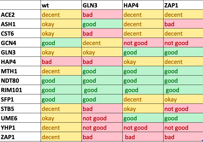
Table 1: The optimized results for were determined to either be a good match, or contrarily a bad match based whether the heat maps shown on GRNmap matched one another or did not. The following are the relationships that were seen: post excel results
Key:
- Bad= colors did not match and were opposite ie one was red and the either was blue across the entire node.
- Not good= Colors did not match in most places of the node.
- Okay= Colors on the heatmap match in certain spots but are opposite in other spots.
- Decent= Shades are not consistent, ie the optimized is light blue and the actual data is dark blue.
- Good= The colors on the heatmap were very close to matching for both the optimized and actual data.
Table 2: Total weights of activation and repression, and Benjamini and Hochberg p-values for each gene

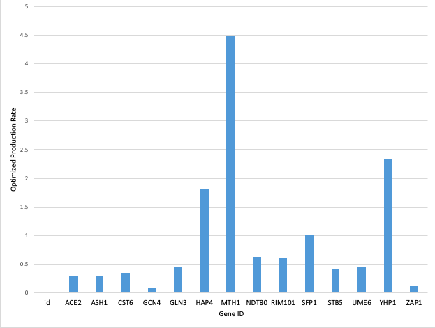
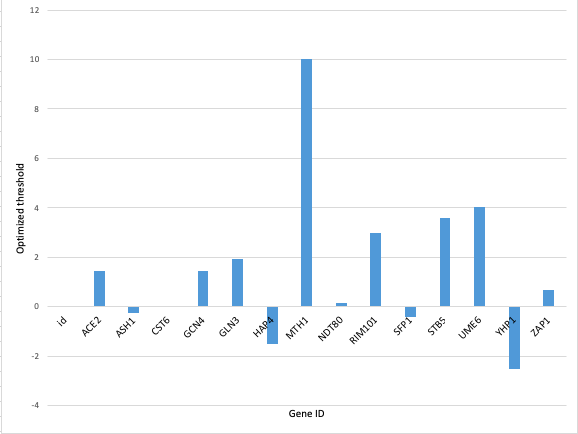
Bar charts representing the optimized b (threshold) and P (production) parameters
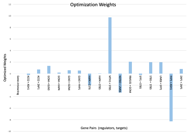
Figure 1: Bar chart displaying the optimized weights per gene interaction which was created as part of the week 6 assignment.
Figure 2: Bar chart displaying the optimized production rates for each gene.
Figure 3: Bar chart displaying the optimized threshold for each gene.
- It does not appear that there is something about these parameters that explains the goodness of fit for the individual genes.
Conclusion
The purpose of the week 7 assignment was to begin analysis of the data that has been collected through the various software including YEASTRACT, GRNsight, and GRNmap. Rather than the computer modeling software telling us the results objectively, this week the analysis was done in a subjective manner. A future in silico experiment will be performed in week 9 in order to hopefully improve the optimized results to better fit the raw data. For the in silico model I will be deleting gene Zap1 which was modeled least accurately in the regulatory matrix which was determined by comparing the optimized with the actual data. Additionally, it only had one edge regulating ACE2, as well as it being a self-regulator so I did not feel that deleting it would change too much in my regulatory network.
Acknowledgements
- I would like to acknowledge my homework partners, Desiree, and Brianna, and Fatimah who worked with the dHAP4 strain along with me.
- Additionally, as usual, Leanne was very helpful via text message with explaining some of the graphs and their meaning.
- Dr. Dahlquist was also helpful in office hours with reassuring me that I was on the right path with identifying which relationships were modeled accurately and which were not represented as well.
- Except for what is noted above, this individual journal entry was completed by me and not copied from another source. Avalekander (talk) 12:31, 5 March 2019 (PST)
References
- Dahlquist, K. & Fitpatrick, B. (2019). "BIOL388/S19: Week 7" Biomathematical Modeling, Loyola Marymount University. Accessed from: Week 7 Assignment Page
Template
- Template: Ava Lekander
- User Page: Ava Lekander
- Journal Entries:
- Assignment Pages:
- Class Journal Pages:
- Biology 388 Home Page: BIOL 388 Class Page


