BIOL388/S19:Week 4
An interim journal entry is due on Thursday, February 14 at midnight PST (Wednesday night/Thursday morning); the finished version is due Thursday, February 21 at midnight PST. See protocol below for stopping point for Week 4 and for the deliverables for Week 4 and Week 5.
Individual Journal Assignment
- Store this journal entry as "username Week 4" (i.e., this is the text to place between the square brackets when you link to this page).
- Create the following set of links. (HINT: These links should all be in your personal template that you created for the Week 1 Assignment; you should then simply invoke your template on each new journal entry.)
- Link to your journal entry from your user page.
- Link back from your journal entry to your user page.
- Link to this assignment from your journal entry.
- Don't forget to add the "BIOL388/S19" category to the end of your wiki page.
Homework Partners
Please meet with your partner (either face-to-face or virtually) at least once when preparing this assignment. Even though you may work together to understand the assignment, your journal assignment must be completed individually. It is not acceptable to do a joint assignment and copy it over to each others' journal page.
- Wild type: Angela and Sahil
- Δgln3: Austin and Leanne
- Δhap4: Desiree, Ava, Brianna, Fatimah
- Δzap1: Alison and Edward
Electronic Lab Notebook
Complete your electronic notebook that gives the details of what you did for the assignment this week. Your notebook entry should contain:
- The purpose: what was the scientific purpose of your investigations?
- Note that this is different than the learning purpose.
- Your workflow or methods: what did you actually do? Give a step by step account.
- There should be enough detail provided so that you or another person could re-do it based solely on your notebook.
- You may copy protocol instructions to your page and modify them as to what you actually did, as long as you provide appropriate attribution in the acknowledgments and references section.
- Take advantage of the electronic nature of the notebook by providing screenshots, links to web pages, etc.
- Your results: the answers to the questions in the protocol, plus any other results you gathered. Your results will include some or all of the following: images, plots, data, and files.
- Note that files left on the Desktop or My Documents or Downloads folders on the Seaver 120 computers will be deleted upon restart of the computers. Files stored on the
T:drive will be saved. However, it is not a good idea to trust that they will be there when you next use the computer. - Thus, it is a critical skill for data and computer literacy to back-up your data and files in at least two ways:
- Upload the files to this wiki.
- Upload the files to Box.
- Back them up on your personal flash drive.
- References to data and files should be made within the methods and results section of your notebook, listed above.
- In addition to these inline links, create a Data and Files section of your notebook to make a list of the files generated in this exercise.
- Note that files left on the Desktop or My Documents or Downloads folders on the Seaver 120 computers will be deleted upon restart of the computers. Files stored on the
- A scientific conclusion: what was your main finding for today's project? Did you fulfill the purpose? Why or why not?
- The Acknowledgments section.
- You must acknowledge your homework partner or team members with whom you worked, giving details of the nature of the collaboration. You should include when and how you met and what content you worked on together. An appropriate statement could be (but is not limited to) the following:
- I worked with my homework partner (give name and link name to their user page) in class. We met face-to-face one time outside of class. We texted/e-mailed/chatted online three times. We worked on the <details> portion of the assignment together.
- Acknowledge anyone else you worked with who was not your assigned partner. This could be Dr. Dahlquist or Dr. Fitzpatrick (for example, via office hours), the TA, other students in the class, or even other students or faculty outside of the class.
- If you copied
wiki syntaxor a particular style from another wiki page, acknowledge that here. Provide the user name of the original page, if possible, and provide a link to the page from which you copied the syntax or style. - If you need to reference content, include the formal citation in your References section (see below).
- You must also include this statement:
- "Except for what is noted above, this individual journal entry was completed by me and not copied from another source."
- Sign your Acknowledgments section with your wiki signature.
- You must acknowledge your homework partner or team members with whom you worked, giving details of the nature of the collaboration. You should include when and how you met and what content you worked on together. An appropriate statement could be (but is not limited to) the following:
- The References section. In this section, you need to provide properly formatted citations to any content that was not entirely of your own devising. This includes, but is not limited to:
- methods
- data
- facts
- images
- documents, including the scientific literature
- Do not include citations/references to sources that you did not use.
- You should include a reference to this week's assignment page.
- The references should be formatted according to the APA guidelines.
Microarray Data Analysis
We will be working on the protocols in class on Tuesday, February 5 and Tuesday, February 12. Whatever you do not finish in class will be homework to be completed by the Week 4 journal deadline.
Before you begin...
Viewing File Extensions
- The Windows 10 operating systems defaults to hiding file extensions. To turn them back on, do the following:
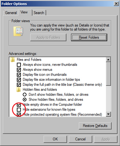
Folder Options window - Go to Cortana (the search function), a circle icon to the right of the start menu and search for "File Explorer Options".
- Open File Explorer Options in the search results.
- When the File Explorer Options window appears, click on the View tab.
- Uncheck the box for "Hide extensions for known file types".
- Click the OK button.
- The computers in Seaver 120 are are set to erase all custom user settings and restore the defaults once they have been restarted, so you will probably have to do this many times throughout the semester when using these computers.

Set Your Browser to Prompt You for the Location to Save your Downloaded Files
- In Mozilla Firefox, open the Options window.
- Select the radio button that says "Always ask you where to save files".
- You could also change the default "Save files to" location to your Desktop, so that will be the first choice when it prompts you where to save the file. (You will have to temporarily deselect the radio button to do this and then reselect it when you are done.
- Click OK to save your changes.
- In Google Chrome, open the Settings window.
- Click on the link at the bottom of the page that says "Advanced Settings".
- Turn on the slider for "Ask where to save each file before downloading".
- You could also change the default Download location to your Desktop, so that will be the first choice when it prompts you where to save the file.
- Your settings are automatically saved.
Background
This is a list of steps required to analyze DNA microarray data.
- Quantitate the fluorescence signal in each spot
- Calculate the ratio of red/green fluorescence
- Log2 transform the ratios
- Steps 1-3 have been performed for you by the GenePix Pro software (which runs the microarray scanner).
- Normalize the ratios on each microarray slide
- Normalize the ratios for a set of slides in an experiment
- Steps 4-5 was performed for you using a script in R, a statistics package (see: Microarray Data Analysis Workflow)
- You will perform the following steps:
- Perform statistical analysis on the ratios
- Compare individual genes with known data
- Steps 6-7 are performed in Microsoft Excel
- Pattern finding algorithms (clustering)
- Map onto biological pathways
- We will use software called STEM for the clustering and mapping
- Identifying regulatory transcription factors responsible for observed changes in gene expression
- Dynamical systems modeling of the gene regulatory network
- The modeling will be performed in MATLAB
For the modeling project, each pair of students will analyze a Dahlquist lab microarray dataset from a particular strain of yeast.
- Wild type: Angela and Sahil
- Δgln3: Austin and Leanne
- Δhap4: Desiree, Ava, Brianna, Fatimah
- Δzap1: Alison and Edward
You will download your assigned Excel spreadsheet from Box. You were e-mailed a link to do this before class. Because the Dahlquist Lab data is unpublished, please do not post it on this public wiki. Instead, post the file(s) back to Box, which is protected by a password.
Experimental Design
In the Excel spreadsheet, there is a worksheet labled "Master_Sheet_<strain>", where strain refers to the particular strain of yeast. In this worksheet, each row contains the data for one gene (one spot on the microarray). The first column contains the "Master Index", which numbers all of the rows sequentially in the worksheet so that we can always use it to sort the genes into the order they were in when we started. The second column (labeled "ID") contains the gene identifier from the Saccharomyces Genome Database. The third column contains the Standard Name for each of the genes. Each subsequent column contains the log2 ratio of the red/green fluorescence from each microarray hybridized in the experiment (steps 1-5 above having been performed for you already).
Each of the column headings from the data begin with the experiment name ("wt" for wild type S. cerevisiae data, "dGLN3" for the Δgln3 data, etc.). "LogFC" stands for "Log2 Fold Change" which is the Log2 red/green ratio. The timepoints are designated as "t" followed by a number in minutes. Replicates are numbered as "-0", "-1", "-2", etc. after the timepoint.
The timepoints are t15, t30, t60 (cold shock at 13°C) and t90 and t120 (cold shock at 13°C followed by 30 or 60 minutes of recovery at 30°C).
- Begin by recording in your wiki, the strain comparison and individual dataset that you will analyze, the filename, the number of replicates for each strain and each time point in your data.
- NOTE: before beginning any analysis, immediately change the filename so that it contains your initials to distinguish it from other students' work.
Statistical Analysis Part 1: ANOVA
The purpose of the witin-stain ANOVA test is to determine if any genes had a gene expression change that was significantly different than zero at any timepoint.
- Create a new worksheet, naming it either "(STRAIN)_ANOVA" as appropriate. For example, you might call yours "wt_ANOVA" or "dHAP4_ANOVA"
- Copy the first three columns containing the "MasterIndex", "ID", and "Standard Name" from the "Master_Sheet" worksheet for your strain and paste it into your new worksheet. Copy the columns containing the data for your strain and paste it into your new worksheet.
- At the top of the first column to the right of your data, create five column headers of the form (STRAIN)_AvgLogFC_(TIME) where (STRAIN) is your strain designation and (TIME) is 15, 30, etc.
- In the cell below the (STRAIN)_AvgLogFC_t15 header, type
=AVERAGE( - Then highlight all the data in row 2 associated with (STRAIN) and t15, press the closing paren key (shift 0),and press the "enter" key.
- This cell now contains the average of the log fold change data from the first gene at t=15 minutes.
- Click on this cell and position your cursor at the bottom right corner. You should see your cursor change to a thin black plus sign (not a chubby white one). When it does, double click, and the formula will magically be copied to the entire column of 6188 other genes.
- Repeat steps (4) through (8) with the t30, t60, t90, and the t120 data.
- Now in the first empty column to the right of the (STRAIN)_AvgLogFC_t120 calculation, create the column header (STRAIN)_ss_HO.
- In the first cell below this header, type
=SUMSQ( - Highlight all the LogFC data in row 2 for your (STRAIN) (but not the AvgLogFC), press the closing paren key (shift 0),and press the "enter" key.
- In the next empty column to the right of (STRAIN)_ss_HO, create the column headers (STRAIN)_ss_(TIME) as in (3).
- Make a note of how many data points you have at each time point for your strain. For most of the strains, it will be 4, but for dHAP4 t90 or t120, it will be "3", and for the wild type it will be "4" or "5". Count carefully. Also, make a note of the total number of data points. Again, for most strains, this will be 20, but for example, dHAP4, this number will be 18, and for wt it should be 23 (double-check).
- In the first cell below the header (STRAIN)_ss_t15, type
=SUMSQ(<range of cells for logFC_t15>)-COUNTA(<range of cells for logFC_t15>)*<AvgLogFC_t15>^2and hit enter.- The
COUNTAfunction counts the number of cells in the specified range that have data in them (i.e., does not count cells with missing values). - The phrase <range of cells for logFC_t15> should be replaced by the data range associated with t15.
- The phrase <AvgLogFC_t15> should be replaced by the cell number in which you computed the AvgLogFC for t15, and the "^2" squares that value.
- Upon completion of this single computation, use the Step (7) trick to copy the formula throughout the column.
- The
- Repeat this computation for the t30 through t120 data points. Again, be sure to get the data for each time point, type the right number of data points, and get the average from the appropriate cell for each time point, and copy the formula to the whole column for each computation.
- In the first column to the right of (STRAIN)_ss_t120, create the column header (STRAIN)_SS_full.
- In the first row below this header, type
=sum(<range of cells containing "ss" for each timepoint>)and hit enter. - In the next two columns to the right, create the headers (STRAIN)_Fstat and (STRAIN)_p-value.
- Recall the number of data points from (13): call that total n.
- In the first cell of the (STRAIN)_Fstat column, type
=((n-5)/5)*(<(STRAIN)_ss_HO>-<(STRAIN)_SS_full>)/<(STRAIN)_SS_full>and hit enter.- Don't actually type the n but instead use the number from (13). Also note that "5" is the number of timepoints and the dSWI4 strain has 4 timepoints (it is missing t15).
- Replace the phrase (STRAIN)_ss_HO with the cell designation.
- Replace the phrase <(STRAIN)_SS_full> with the cell designation.
- Copy to the whole column.
- In the first cell below the (STRAIN)_p-value header, type
=FDIST(<(STRAIN)_Fstat>,5,n-5)replacing the phrase <(STRAIN)_Fstat> with the cell designation and the "n" as in (13) with the number of data points total. (Again, note that the number of timepoints is actually "4" for the dSWI4 strain). Copy to the whole column. - Before we move on to the next step, we will perform a quick sanity check to see if we did all of these computations correctly.
- Click on cell A1 and click on the Data tab. Select the Filter icon (looks like a funnel). Little drop-down arrows should appear at the top of each column. This will enable us to filter the data according to criteria we set.
- Click on the drop-down arrow on your (STRAIN)_p-value column. Select "Number Filters". In the window that appears, set a criterion that will filter your data so that the p value has to be less than 0.05.
- Excel will now only display the rows that correspond to data meeting that filtering criterion. A number will appear in the lower left hand corner of the window giving you the number of rows that meet that criterion. We will check our results with each other to make sure that the computations were performed correctly.
Calculate the Bonferroni and p value Correction
- Now we will perform adjustments to the p value to correct for the multiple testing problem. Label the next two columns to the right with the same label, (STRAIN)_Bonferroni_p-value.
- Type the equation
=<(STRAIN)_p-value>*6189, Upon completion of this single computation, use the Step (10) trick to copy the formula throughout the column. - Replace any corrected p value that is greater than 1 by the number 1 by typing the following formula into the first cell below the second (STRAIN)_Bonferroni_p-value header:
=IF(STRAIN_Bonferroni_p-value>1,1,STRAIN_Bonferroni_p-value), where "STRAIN_Bonferroni_p-value" refers to the cell in which the first Bonferroni p value computation was made. Use the Step (10) trick to copy the formula throughout the column.
Calculate the Benjamini & Hochberg p value Correction
- Insert a new worksheet named "(STRAIN)_ANOVA_B-H".
- Copy and paste the "MasterIndex", "ID", and "Standard Name" columns from your previous worksheet into the first two columns of the new worksheet.
- For the following, use Paste special > Paste values. Copy your unadjusted p values from your ANOVA worksheet and paste it into Column D.
- Select all of columns A, B, C, and D. Sort by ascending values on Column D. Click the sort button from A to Z on the toolbar, in the window that appears, sort by column D, smallest to largest.
- Type the header "Rank" in cell E1. We will create a series of numbers in ascending order from 1 to 6189 in this column. This is the p value rank, smallest to largest. Type "1" into cell E2 and "2" into cell E3. Select both cells E2 and E3. Double-click on the plus sign on the lower right-hand corner of your selection to fill the column with a series of numbers from 1 to 6189.
- Now you can calculate the Benjamini and Hochberg p value correction. Type (STRAIN)_B-H_p-value in cell F1. Type the following formula in cell F2:
=(D2*6189)/E2and press enter. Copy that equation to the entire column. - Type "STRAIN_B-H_p-value" into cell G1.
- Type the following formula into cell G2:
=IF(F2>1,1,F2)and press enter. Copy that equation to the entire column. - Select columns A through G. Now sort them by your MasterIndex in Column A in ascending order.
- Copy column G and use Paste special > Paste values to paste it into the next column on the right of your ANOVA sheet.
- Upload the .xlsx file that you have just created to Box. Send Dr. Dahlquist and Dr. Fitzpatrick an e-mail with the link to the file (e-mail kdahlquist or bfitzpatrick at lmu dot edu).
Sanity Check: Number of genes significantly changed
Before we move on to further analysis of the data, we want to perform a more extensive sanity check to make sure that we performed our data analysis correctly. We are going to find out the number of genes that are significantly changed at various p value cut-offs.
- Go to your (STRAIN)_ANOVA worksheet.
- Select row 1 (the row with your column headers) and select the menu item Data > Filter > Autofilter (The funnel icon on the Data tab). Little drop-down arrows should appear at the top of each column. This will enable us to filter the data according to criteria we set.
- Click on the drop-down arrow for the unadjusted p value. Set a criterion that will filter your data so that the p value has to be less than 0.05.
- How many genes have p < 0.05? and what is the percentage (out of 6189)?
- How many genes have p < 0.01? and what is the percentage (out of 6189)?
- How many genes have p < 0.001? and what is the percentage (out of 6189)?
- How many genes have p < 0.0001? and what is the percentage (out of 6189)?
- When we use a p value cut-off of p < 0.05, what we are saying is that you would have seen a gene expression change that deviates this far from zero by chance less than 5% of the time.
- We have just performed 6189 hypothesis tests. Another way to state what we are seeing with p < 0.05 is that we would expect to see this a gene expression change for at least one of the timepoints by chance in about 5% of our tests, or 309 times. Since we have more than 309 genes that pass this cut off, we know that some genes are significantly changed. However, we don't know which ones. To apply a more stringent criterion to our p values, we performed the Bonferroni and Benjamini and Hochberg corrections to these unadjusted p values. The Bonferroni correction is very stringent. The Benjamini-Hochberg correction is less stringent. To see this relationship, filter your data to determine the following:
- How many genes are p < 0.05 for the Bonferroni-corrected p value? and what is the percentage (out of 6189)?
- How many genes are p < 0.05 for the Benjamini and Hochberg-corrected p value? and what is the percentage (out of 6189)?
- In summary, the p value cut-off should not be thought of as some magical number at which data becomes "significant". Instead, it is a moveable confidence level. If we want to be very confident of our data, use a small p value cut-off. If we are OK with being less confident about a gene expression change and want to include more genes in our analysis, we can use a larger p value cut-off.
- Comparing results with known data: the expression of the gene NSR1 (ID: YGR159C)is known to be induced by cold shock. Find NSR1 in your dataset. What is its unadjusted, Bonferroni-corrected, and B-H-corrected p values? What is its average Log fold change at each of the timepoints in the experiment? Note that the average Log fold change is what we called "STRAIN)_AvgLogFC_(TIME)" in step 3 of the ANOVA analysis.
- We will compare the numbers we get between the wild type strain and the other strains studied, organized as a table. Use this sample PowerPoint slide to see how your table should be formatted. (Note that you will need to unzip the file after downloading.)
Stopping point for the Week 4 Assignment
Clustering and GO Term Enrichment with stem (part 2)
- Prepare your microarray data file for loading into STEM. Have this part completed for Tuesday, February 19.
- Insert a new worksheet into your Excel workbook, and name it "(STRAIN)_stem".
- Select all of the data from your "(STRAIN)_ANOVA" worksheet and Paste special > paste values into your "(STRAIN)_stem" worksheet.
- Your leftmost column should have the column header "Master_Index". Rename this column to "SPOT". Column B should be named "ID". Rename this column to "Gene Symbol". Delete the column named "Standard_Name".
- Filter the data on the B-H corrected p value to be > 0.05 (that's greater than in this case).
- Once the data has been filtered, select all of the rows (except for your header row) and delete the rows by right-clicking and choosing "Delete Row" from the context menu. Undo the filter. This ensures that we will cluster only the genes with a "significant" change in expression and not the noise.
- Delete all of the data columns EXCEPT for the Average Log Fold change columns for each timepoint (for example, wt_AvgLogFC_t15, etc.).
- Rename the data columns with just the time and units (for example, 15m, 30m, etc.).
- Save your work. Then use Save As to save this spreadsheet as Text (Tab-delimited) (*.txt). Click OK to the warnings and close your file.
- Note that you should turn on the file extensions if you have not already done so.
- Now download and extract the STEM software. Click here to go to the STEM web site.
- Click on the download link and download the
stem.zipfile to your Desktop. - Unzip the file. In Seaver 120, you can right click on the file icon and select the menu item 7-zip > Extract Here.
- This will create a folder called
stem.- You now need to download the Gene Ontology and yeast GO annotations and place them in this folder.
- Click here to download the file "gene_ontology.obo".
- Click here to download the file "gene_association.sgd.gz".
- Inside the folder, double-click on the
stem.jarto launch the STEM program.
- Click on the download link and download the
- Running STEM
- In section 1 (Expression Data Info) of the the main STEM interface window, click on the Browse... button to navigate to and select your file.
- Click on the radio button No normalization/add 0.
- Check the box next to Spot IDs included in the data file.
- In section 2 (Gene Info) of the main STEM interface window, leave the default selection for the three drop-down menu selections for Gene Annotation Source, Cross Reference Source, and Gene Location Source as "User provided".
- Click the "Browse..." button to the right of the "Gene Annotation File" item. Browse to your "stem" folder and select the file "gene_association.sgd.gz" and click Open.
- In section 3 (Options) of the main STEM interface window, make sure that the Clustering Method says "STEM Clustering Method" and do not change the defaults for Maximum Number of Model Profiles or Maximum Unit Change in Model Profiles between Time Points.
- In section 4 (Execute) click on the yellow Execute button to run STEM.
- In section 1 (Expression Data Info) of the the main STEM interface window, click on the Browse... button to navigate to and select your file.
- Viewing and Saving STEM Results
- A new window will open called "All STEM Profiles (1)". Each box corresponds to a model expression profile. Colored profiles have a statistically significant number of genes assigned; they are arranged in order from most to least significant p value. Profiles with the same color belong to the same cluster of profiles. The number in each box is simply an ID number for the profile.
- Click on the button that says "Interface Options...". At the bottom of the Interface Options window that appears below where it says "X-axis scale should be:", click on the radio button that says "Based on real time". Then close the Interface Options window.
- Take a screenshot of this window (on a PC, simultaneously press the
AltandPrintScreenbuttons to save the view in the active window to the clipboard) and paste it into a PowerPoint presentation to save your figures.
- Click on each of the SIGNIFICANT profiles (the colored ones) to open a window showing a more detailed plot containing all of the genes in that profile.
- Take a screenshot of each of the individual profile windows and save the images in your PowerPoint presentation.
- At the bottom of each profile window, there are two yellow buttons "Profile Gene Table" and "Profile GO Table". For each of the profiles, click on the "Profile Gene Table" button to see the list of genes belonging to the profile. In the window that appears, click on the "Save Table" button and save the file to your desktop. Make your filename descriptive of the contents, e.g. "wt_profile#_genelist.txt", where you replace the number symbol with the actual profile number.
- Upload these files to OpenWetWare and link to them on your individual journal page. (Note that it will be easier to zip all the files together and upload them as one file).
- For each of the significant profiles, click on the "Profile GO Table" to see the list of Gene Ontology terms belonging to the profile. In the window that appears, click on the "Save Table" button and save the file to your desktop. Make your filename descriptive of the contents, e.g. "wt_profile#_GOlist.txt", where you use "wt", "dGLN3", etc. to indicate the dataset and where you replace the number symbol with the actual profile number. At this point you have saved all of the primary data from the STEM software and it's time to interpret the results!
- Upload these files to OpenWetWare and link to them on your individual journal page. (Note that it will be easier to zip all the files together and upload them as one file).
- A new window will open called "All STEM Profiles (1)". Each box corresponds to a model expression profile. Colored profiles have a statistically significant number of genes assigned; they are arranged in order from most to least significant p value. Profiles with the same color belong to the same cluster of profiles. The number in each box is simply an ID number for the profile.
- Analyzing and Interpreting STEM Results
- Select one of the profiles you saved in the previous step for further intepretation of the data. I suggest that you choose one that has a pattern of up- or down-regulated genes at the cold shock timepoints. Each member of your group should choose a different profile. Answer the following:
- Why did you select this profile? In other words, why was it interesting to you?
- How many genes belong to this profile?
- How many genes were expected to belong to this profile?
- What is the p value for the enrichment of genes in this profile? Bear in mind that we just finished computing p values to determine whether each individual gene had a significant change in gene expression at each time point. This p value determines whether the number of genes that show this particular expression profile across the time points is significantly more than expected.
- Open the GO list file you saved for this profile in Excel. This list shows all of the Gene Ontology terms that are associated with genes that fit this profile. Select the third row and then choose from the menu Data > Filter > Autofilter. Filter on the "p-value" column to show only GO terms that have a p value of < 0.05. How many GO terms are associated with this profile at p < 0.05? The GO list also has a column called "Corrected p-value". This correction is needed because the software has performed thousands of significance tests. Filter on the "Corrected p-value" column to show only GO terms that have a corrected p value of < 0.05. How many GO terms are associated with this profile with a corrected p value < 0.05?
- Select 6 Gene Ontology terms from your filtered list (either p < 0.05 or corrected p < 0.05).
- Each member of the group will be reporting on his or her own cluster in your research presentation. You should take care to choose terms that are the most significant, but that are also not too redundant. For example, "RNA metabolism" and "RNA biosynthesis" are redundant with each other because they mean almost the same thing.
- Note whether the same GO terms are showing up in multiple clusters.
- Look up the definitions for each of the terms at http://geneontology.org. In your research presentation, you will discuss the biological interpretation of these GO terms. In other words, why does the cell react to cold shock by changing the expression of genes associated with these GO terms? Also, what does this have to do with the transcription factor being deleted (for the Δgln3 and Δswi4 groups)?
- To easily look up the definitions, go to http://geneontology.org.
- Copy and paste the GO ID (e.g. GO:0044848) into the search field on the left of the page.
- In the results page, click on the button that says "Link to detailed information about <term>, in this case "biological phase"".
- The definition will be on the next results page, e.g. here.
- Each member of the group will be reporting on his or her own cluster in your research presentation. You should take care to choose terms that are the most significant, but that are also not too redundant. For example, "RNA metabolism" and "RNA biosynthesis" are redundant with each other because they mean almost the same thing.
- Select one of the profiles you saved in the previous step for further intepretation of the data. I suggest that you choose one that has a pattern of up- or down-regulated genes at the cold shock timepoints. Each member of your group should choose a different profile. Answer the following:
Using YEASTRACT to Infer which Transcription Factors Regulate a Cluster of Genes (Tuesday, Feb. 19)
In the previous analysis using STEM, we found a number of gene expression profiles (aka clusters) which grouped genes based on similarity of gene expression changes over time. The implication is that these genes share the same expression pattern because they are regulated by the same (or the same set) of transcription factors. We will explore this using the YEASTRACT database.
- Open the gene list in Excel for the one of the significant profiles from your stem analysis. Choose a cluster with a clear cold shock/recovery up/down or down/up pattern. You should also choose one of the largest clusters.
- Copy the list of gene IDs onto your clipboard.
- Launch a web browser and go to the YEASTRACT database.
- On the left panel of the window, click on the link to Rank by TF.
- Paste your list of genes from your cluster into the box labeled ORFs/Genes.
- Check the box for Check for all TFs.
- Accept the defaults for the Regulations Filter (Documented, DNA binding plus expression evidence)
- Do not apply a filter for "Filter Documented Regulations by environmental condition".
- Rank genes by TF using: The % of genes in the list and in YEASTRACT regulated by each TF.
- Click the Search button.
- Answer the following questions:
- In the results window that appears, the p values colored green are considered "significant", the ones colored yellow are considered "borderline significant" and the ones colored pink are considered "not significant". How many transcription factors are green or "significant"?
- Copy the table of results from the web page and paste it into a new Excel workbook to preserve the results.
- Upload the Excel file to OWW or Box and link to it in your electronic lab notebook.
- Are GLN3, HAP4, and/or ZAP1 on the list? If so, what is their "% in user set", "% in YEASTRACT", and "p value".
- For the mathematical model that we will build, we need to define a gene regulatory network of transcription factors that regulate other transcription factors. We can use YEASTRACT to assist us with creating the network. We want to generate a network with approximately 15-20 transcription factors in it.
- You need to select from this list of "significant" transcription factors, which ones you will use to run the model. You will use these transcription factors and add GLN3, HAP4, and ZAP1 if they are not in your list. Explain in your electronic notebook how you decided on which transcription factors to include. Record the list and your justification in your electronic lab notebook. Each group member will select a different network (they can have some overlapping transcription factors, but some should also be different).
- Go back to the YEASTRACT database and follow the link to Generate Regulation Matrix.
- Copy and paste the list of transcription factors you identified (plus HAP4, GLN3, and ZAP1) into both the "Transcription factors" field and the "Target ORF/Genes" field.
- We are going to use the "Regulations Filter" options of "Documented", "Only DNA binding evidence"
- Click the "Generate" button.
- In the results window that appears, click on the link to the "Regulation matrix (Semicolon Separated Values (CSV) file)" that appears and save it to your Desktop. Rename this file with a meaningful name so that you can distinguish it from the other files you will generate.
Visualizing Your Gene Regulatory Networks with GRNsight (Tuesday, Feb. 19)
We will analyze the regulatory matrix files you generated above in Microsoft Excel and visualize them using GRNsight to determine which one will be appropriate to pursue further in the modeling.
- First we need to properly format the output files from YEASTRACT.
- Open the file in Excel. It will not open properly in Excel because a semicolon was used as the column delimiter instead of a comma. To fix this, Select the entire Column A. Then go to the "Data" tab and select "Text to columns". In the Wizard that appears, select "Delimited" and click "Next". In the next window, select "Semicolon", and click "Next". In the next window, leave the data format at "General", and click "Finish". This should now look like a table with the names of the transcription factors across the top and down the first column and all of the zeros and ones distributed throughout the rows and columns. This is called an "adjacency matrix." If there is a "1" in the cell, that means there is a connection between the trancription factor in that row with that column.
- Save this file in Microsoft Excel workbook format (.xlsx).
- For this adjacency matrix to be usable in GRNmap (the modeling software) and GRNsight (the visualization software), we need to transpose the matrix. Insert a new worksheet into your Excel file and name it "network". Go back to the previous sheet and select the entire matrix and copy it. Go to you new worksheet and click on the A1 cell in the upper left. Select "Paste special" from the "Home" tab. In the window that appears, check the box for "Transpose". This will paste your data with the columns transposed to rows and vice versa. This is necessary because we want the transcription factors that are the "regulatORS" across the top and the "regulatEES" along the side.
- The labels for the genes in the columns and rows need to match. Thus, delete the "p" from each of the gene names in the columns. Adjust the case of the labels to make them all upper case.
- In cell A1, copy and paste the text "rows genes affected/cols genes controlling".
- Finally, for ease of working with the adjacency matrix in Excel, we want to alphabatize the gene labels both across the top and side.
- Select the area of the entire adjacency matrix.
- Click the Data tab and click the custom sort button.
- Sort Column A alphabetically, being sure to exclude the header row.
- Now sort row 1 from left to right, excluding cell A1. In the Custom Sort window, click on the options button and select sort left to right, excluding column 1.
- Name the worksheet containing your organized adjacency matrix "network" and Save.
- Now we will visualize what these gene regulatory networks look like with the GRNsight software.
- Go to the GRNsight home page.
- Select the menu item File > Open and select the regulation matrix .xlsx file that has the "network" worksheet in it that you formatted above. If the file has been formatted properly, GRNsight should automatically create a graph of your network. You can click the "Grid Layout" button to arrange the nodes in a grid, or you can click and drag the nodes (genes) around until you get a layout that you like and take a screenshot of the results. Paste it into your PowerPoint presentation.
- If you have nodes (genes) floating around in the display that are not connected to any other nodes, we need to delete them from the network for the modeling to work properly. Go back to the Excel workbook and network sheet and delete both the row and column with the floating gene's name. Then re-upload the edited file to GRNsight to visualize it. Use this final version in your PowerPoint and subsequent modeling.
Summary of what you need to turn in for the individual Weeks 4 and 5 assignments
You will continue working on your Week 4 individual journal page for the Week 5 assignment as well. The two assignments will be graded together after the Week 5 due date for 20 points, instead of individually for 10 points each.
By the Week 4 deadline, submit:
- Your individual journal page should have an electronic lab notebook recording your work for this week. This includes the purpose, detailed methods, your results, the answers to any questions posed in the protocol above, a scientific conclusion, and the acknowledgments and references sections. You are responsible for completing the procedure up to the designated stopping point.
- Upload your updated Excel spreadsheet to Box that has today's calculations in it. Use the same filename as before so that the download link that you already provided to Drs. Dahlquist and Fitzpatrick will still work.
- Create, upload to OpenWetWare, and link to a PowerPoint presentation that contains the p value table. You will need to zip it because OWW does not accept .ppt or .pptx as a file format anymore.
By the Week 5 deadline, submit:
- Continuation of the individual journal page for Week 4 with your electronic lab notebook recording your work for the last two weeks. This includes the purpose, detailed methods, your results, the answers to any questions posed in the protocol above, a scientific conclusion, and the acknowledgments and references sections. You will add to what you submitted to the interim deadline on Week 4. Don't forget your paragraph which is a biological interpretation of your stem results.
- Add the screenshots of your stem results and GRNsight visualization to the PowerPoint file from last week. Do not change the filename, just upload a newer version of the file. Each slide in the presentation should have a meaningful title that describes the main message of the slide. These slides will form the basis of your research presentation for this project.
- Zip together all of the tab-delimited text files that you created for and from stem and upload them to Box:
- the .txt file that was saved from your original spreadsheet that you used to run stem
- each of the genelist and GOlist files for each of your significant profiles.
- You will have a revised version of the main data analysis Excel workbook with additional sheets for the stem input, YEASTRACT rank by TF output, and GRNsight network.
- The shared journal assignment below.
Shared Journal Assignment
The shared journal assignment will be due on the Week 5 deadline, midnight, February 21 (Wednesday night/Thursday morning).
- Store your shared journal entry in the shared Class Journal Week 4 page. If this page does not exist yet, go ahead and create it (congratulations on getting in first :) )
- Link to your journal entry from your user page.
- Link back from the journal entry to your user page.
- Sign your portion of the journal with the standard wiki signature shortcut (
~~~~). - Add the "BIOL388/S19" category to the end of the wiki page (if someone has not already done so).
View
Now that you've done your own microarray data analysis, we will revisit the case "Deception at Duke".
- View the video: The Importance of Reproducible Research in High-Throughput Biology: Case Studies in Forensic Bioinformatics. Here is an alternate link to the video.
- View the slides from DataONE on data entry and manipulation.
- Optional: for more information on the Duke saga, see the web site put together by Baggerly and Coombes here.
Reflection
- What were the main issues with the data and analysis identified by Baggerly and Coombs? What best practices enumerated by DataONE were violated? Which of these did Dr. Baggerly claim were common issues?
- What recommendations does Dr. Baggerly recommend for reproducible research? How do these correspond to what DataONE recommends?
- Do you have any further reaction to this case after viewing Dr. Baggerly's talk?
- Go back to the methods section of the paper you presented for journal club. Do you think there is sufficient information there to reproduce their data analysis? Why or why not?
