Avalekander Week 11: Difference between revisions
From OpenWetWare
Jump to navigationJump to search
Avalekander (talk | contribs) |
Avalekander (talk | contribs) →Background: changed wording around |
||
| Line 18: | Line 18: | ||
*qu= inflow rate | *qu= inflow rate | ||
*qy(t)= outflow rate | *qy(t)= outflow rate | ||
* | *consumption rate/rate of metabolism: qu-qy(t)-(Er(y/K + y)x(t) | ||
*x= yeast cell concentration | *x= yeast cell concentration | ||
*E= unit conversion rate between biomass (the units of x) and nutrient concentration | *E= unit conversion rate between biomass (the units of x) and nutrient concentration | ||
Revision as of 22:28, 10 April 2019
Purpose
- The purpose of this assignment is using MatLab to simulate a chemostat through the use of differential equations and then making a graphical representation. Then the values formulated will be compared with hand calculations in order to determine if the results for the steady state are the same.
Background
- The chemostat is an idealized environment for displaying the growth of yeast populations.
- Nutrients are fed continuously in the chemostat at a fixed flow rate and concentration, and effluent is extracted at a fixed flow rate as well.
- It can be assumed that the contents of the chemostat are thoroughly mixed and that concentrations are uniform throughout.
- The parameters below are based on this assumption that all yeast cells have equal access to nutrients.
- u= feed concentration (mass or molar)
- q= dilution rate (1/time)
- Q=volumetric inflow rate (vol/time)
- V= volume of the mixture in the tank (constant)
- y(t)= concentration of nutrients
Rate of change of nutrient = inflow rate – outflow rate – rate consumed in the tank.
- The model of consumption is called Michaelis-Menten:
- qu= inflow rate
- qy(t)= outflow rate
- consumption rate/rate of metabolism: qu-qy(t)-(Er(y/K + y)x(t)
- x= yeast cell concentration
- E= unit conversion rate between biomass (the units of x) and nutrient concentration
- r= Maximum rate of system (Vmax)
- K= Nutrient concentration at which the reaction rate is half of Vmax (r)
- At equilibrium the equations are set to zero
- x cannot equal zero though
- Nutrient concentration at zero: y=qK/(r-q)
- Cell concentration at zero: x=(u-y)/E
- The steady state nutrient concentration is independent of the feed rate u, while the cell population depends linearly on u
Methods
- This file was read and used for background information: Chemostat Modeling Assignment.
- The MATLAB files named chemostat_script.m and chemostat_dynamics.m were used to simulate a chemostat and compare the computations to a steady state outcome.
- The following is the zip file used: here
- The parameter values used were:
- q = 0.10 (1/hr)
- u = 5 (g/L)
- E = 1.5
- r = 0.8 (1/hr)
- K = 8 (g)
- The parameter values were plugged into the following equations to formulate the steady states of cell biomass and nutrient mass:
- y = qK/(r-q)
- x = (u-y)/E
- Assuming a 2 liter chemostat, the steady state concentrations of cells and nutrients were then calculated by dividing the previous values found for x and y by 2 L.
- The system dynamics were simulated using the MATLAB files and the parameters of (1).
- After simulating the graph I will then determine if the graphs show the system going to steady state and whether the steady states in the graph match the calculations performed by hand.
- BONUS: can you get two y-axes, with the second one to the right of the picture like in the journal articles you’ve read?
Results
- Parameters were plugged into y = qK/(r-q) and x = (u-y)/E to solve for cell biomass and nutrient mass (g) at equilibrium
- Nutrient mass- y=(0.1(8))/(0.8-0.1)=1.14 g
- Cell biomass- x=(5-1.14)/1.5 = 2.6 g
- Concenration in a 2L chemostat:
- Nutrient mass = 1.14g/2L = 0.55 g/L
- Cell biomass = 2.6g/L = 1.3 g/L
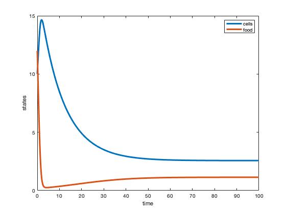
- MatLab Simulation:
Fig. 1: The figure above shows time on the x-axis and states on the y-axis for both grams of nutrient and grams of cells present. At around 50 hours equilibrium or steady state has been reached.
- Yes, the figure does show the system going to steady state around the 50 hour mark in which the lines representing cells and nutrients appear to plateau or seem to reach equilibrium.
- Yes, the graphs do appear to match my calculations as you can see that around the 50 hour mark nutrient levels appear to be at around 1 grams and cells appear to be around 3 grams.
Conclusion
- The graph simulated through MatLab shows that the steady state is reached at around 40-50 hours and the values shown in the graph match the calculations I performed by hand.
Acknowledgements
- I would like to acknowledge my homework partner, Edward with whom I worked with to complete the assignment.
- Additionally, I would like to acknowledge Leanne with whom I communicated with via text message when I was confused about the MatLab script versus dynamic files and where the parameter values should be plugged in.
- I would also like to acknowledge Dr. Dahlquist, as well as Dr. Fitzpatrick for their help throughout the assignment.
Except for what is noted above, this individual journal entry was completed by me and not copied from another source. Avalekander (talk) 14:19, 9 April 2019 (PDT)
References
- Dahlquist, K. & Fitpatrick, B. (2019). "BIOL388/S19: Week 11" Biomathematical Modeling, Loyola Marymount University. Accessed from:Week 11 Assignment Page
Biology 388 Assignments
- Template: Ava Lekander
- User Page: Ava Lekander
- Journal Entries:
- Assignment Pages:
- Class Journal Pages:
- Biology 388 Home Page: BIOL 388 Class Page
