Sahil Patel Week 7

Electronic Lab Notebook

Purpose

The purpose of this assignment was to understand the data included in the output Excel workbook by analyzing the optimized values returned from the MATLAB program as well as to propose further experimentation that could lead to interesting results.

Methods

Analyzing Results of First Model Run

The output workbook that was created last week was used to identify the least squares error (LSE) for our model.
On the "optimization_diagnostics" worksheet, the LSE:minLSE ratios for the ten models run by everyone in the class were compared and analyzed.
The output Excel workbook was then uploaded to GRNsight and the the actual data for a strain was compared with the simulated data from the same strain to see where there was a good fit versus a bad fit.
A table was created to organize the genes along with their respective number of incoming arrows, Benjamini & Hochberg corrected p-value, and the relative change of gene expression.
Bar charts were created for the b and P parameters to give additional insight on the goodness of fit for the individual genes.

Tweaking the Model and Analyzing the Results

To proceed with the in silico experiment, my homework partner Angela and I discussed possible ideas that we could "tweak" to the original protocol.
Ideas were given by Dr. Dahlquist in order to steer us in the right direction; these included:

In our initial runs, we estimated all three parameters w, P, and b.
- How do the modeling results change if P is instead fixed and w and b are estimated?
- How do the modeling results change if b is fixed and w and P are estimated?
- How do the modeling results change if P and b are fixed, and only w is estimated?
For our initial runs, we included all three microarray datasets, wt, Δgln3, and Δhap4.
- What happens to the results if we base the estimation on just two strains (wt + one deletion strain)?
- What happens to the results if we base the estimation on just the wt strain data?
When viewing the modeling results in GRNsight, you may determine that one or more genes in the network does not appear to be doing much.
- What happens to the modeling results if you delete this gene from the network and re-run the model (remember you will have to delete references to this gene in all worksheets of the input file).
You also might think that a particular edge (regulatory relationship) is not needed. What happens if you delete that edge?
What happens if you include the t90 and t120 expression data?

Results

Protocol Questions

What is the overall least squares error (LSE) for your model?
- 0.706826034
What is the LSE to minLSE ratio?
- LSE/minLSE = 0.706826034/0.496201197 = 1.424474665
Which genes are modeled well?
- ACE2
- ERT1
- GCR1
- HAP2
- GLN3
Which genes are not modeled well?
- HAP4
- LEU3
- MGA2
- STB5
- SUM1
- ZAP1
What is the ANOVA Benjamini & Hochberg corrected p value for the gene?
Is the gene changing its expression a lot or is the log2 fold change mostly near zero?

Table 1. Genes including rows with respective number of incoming arrows, Benjamini & Hochberg corrected p-value, and the relative change of gene expression.

What explains the goodness of fit to the model?
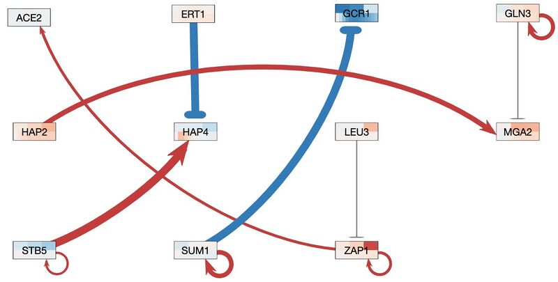
- The color of the top half of a node will match or follow a close enough trend as the bottom half of each gene in a good fit. Likewise, if the colors do not match then it is a poor fit. The intensity or boldness of the color plays a factor as well.

Figures and Data

To access the optimization diagnostic as well as the individual expression plots produced by MATLAB click here.
To view the output Excel workbook produced from MATLAB, click here.
The Final Powerpoint Presentation is linked here.

Figure 1. The gene map produced by GRNsight displayed 11 nodes and 11 edges. The top half of the node was set to wt_log2_expression while the bottom half was set to wt_log2_optimized_expression using the average replicate values for both. The log fold change maximum value was left at 3.

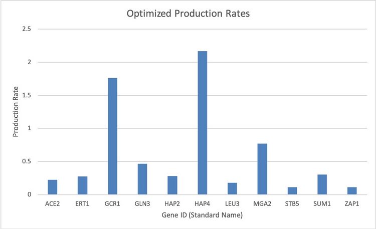
Figure 2. This bar graph represents the optimized production rates (P) of the genes as per the output Excel workbook.

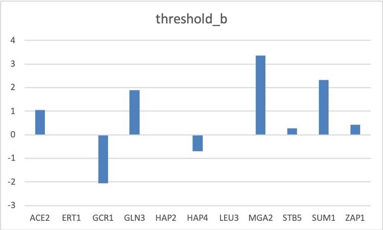
Figure 3. This bar graph represents the optimized threshold_b values (b) of the genes as per the output Excel workbook.

Conclusion

In this experiment, we analyzed the goodness of fit of the model created through the MATLAB program and used that to compare gene expression changes. After analyzing the data, it is believed that there is no coorelation or significant data based on the optimized production rates and the optimized threshold_b. For our in silico experiment my partner and I have chosen to keep the genes that were originally deleted from the GRNsight network because they were disconnected nodes.

Acknowledgments

Angela Abarquez, and I communicated in class and via text for clarifications regarding the tweak we would make in our methods for the in silico experiment. Except for what is noted above, this individual journal entry was completed by me and not copied from another source.

Sahil Patel (talk) 06:10, 19 March 2019 (PDT)