EdwardRyanTalatala Week 7
Purpose
The purpose of this assignment is to analyze the results of the GNRmap workbook on GRNsight. GRNsight created the model of how the gene clusters interacted, depicting which genes were activated or repressed through proportionally sized arrows and colors.
Methods
Analyzing Results of First Model Run
Here is what you need to consider when analyzing the results of your model.
- What is the overall least squares error (LSE) for your model?
- You will find this on the "optimization_diagnostics" worksheet of your output workbook.
- Since the input data are noisy, the model can only minimize the error so far. It is more "fair" to look at the ratio of the least squares error to the minimum theoretical least squares error that the model could have achieved given the data. We call this the LSE:minLSE ratio. You should be able to compute it with the values given on the "optimization_diagnostics" worksheet.
- We will compare the LSE:minLSE ratios for the ten models run by everyone in the class.
- You need to look at the individual fits for each of the genes in your model. Which genes are modeled well? Which genes are not modeled well?
- Look at the individual expression plots to see if the line that represents the simulated model data is a good fit to the individual data points.
- Upload your output Excel spreadsheet to GRNsight. Use the dropdown menu on the left to choose the data you will display on the nodes (boxes). Compare the actual data for a strain with the simulated data from the same strain. If the model fits the data well, the color heatmap superimposed on the node will match top and bottom. If the fit is less good, the colors will not match.
- What explains the goodness of fit to the model?
- How many arrows are incoming to the node?
- What is the ANOVA Benjamini & Hochberg corrected p value for the gene?
- Is the gene changing its expression a lot or is the log2 fold change mostly near zero?
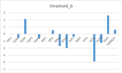
- Make bar charts for the b and P parameters.
- Is there something about these parameters that explains the goodness of fit for the individual genes?
Tweaking the Model and Analyzing the Results
We will carry out an additional in silico experiment with our model. We will report out our results in a research presentation in Week 9.
- For our initial runs, we estimated all three parameters w, P, and b. We want to see:
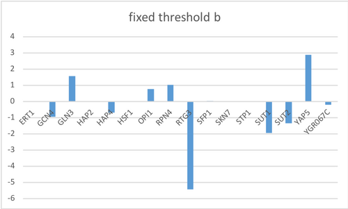
- How do the modeling results change if b is fixed and w and P are estimated?
- This might be interesting because the current b values vary so much between each gene. I think that fixing b will create very different model results.
- To choose our fixed b values, we are going to sum up the weights of the controllers of each gene and use that value as b.
- Do this by summing up the rows in the network_optimized_weights sheet.
- Change these values threshold_b worksheet in the GRNmap input workbook
- In the Optimization Parameters worksheet, change threshold_b value to 1 to fix this parameter
Results
New GRNmap run with new workbook
- Overall least squares error (LSE): 0.720128194
- LSE:minLSE ratio: 1.307
- Individual fits of GRNsight models
- wild type
- HAP4 has opposite expression
- All other genes show relatively the same expression
- dgln3
- SKN7 optimized data does not show strong activation compared to actual data
- All other genes show relatively the same expression
- dhap4
- All nodes look relatively the same between actual and optimized data.
- wild type
New GRNmap run with Fixed Threshold B
- Overall least squares error (LSE): 0.726836138
- LSE:minLSE ratio: 1.32
- GRNsight models after fixing Threshold B
- wild type
- All nodes look relatively the same between actual and optimized data.
- dgln3
- SKN7 optimized data does not show strong activation compared to actual data
- All other genes show relatively the same expression
- dhap4
- All nodes look relatively the same between actual and optimized data.
- wild type
Conclusion
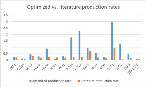
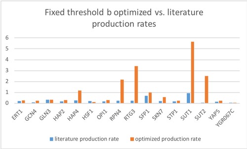
Due to the bug when I ran GRNsight, I could not do the second part of "Analyzing Results of First Model Run," determine goodness of fit for the genes. However, I was able to do the first and third parts. I found the LSE of my GRNmap was 2.1698, while my LSE:minLSE ratio was 1.2447. As for the production rates of my results, nearly all of the optimized production rates had a greater value than that of the literature, the exception being gene YGR067G. However, both values were very similar, the difference in valuable is negligible. The genes with the greatest differences in values are HAP4, RPN4, RTG3, SUT1, SUT2, & YAP5.
After using the new GRNmap input workbook without any bugs, the model seems to fit well for predicting the expression of genes due to the fact that only a few nodes did not match with the optimized and actual data. Even after fixing the threshold b parameter, the resulting GRNsight gene cluster did not change much. This may be because the LSE and LSE:minLSE ratio were relatively the same.
Acknowledgments
I worked with my homework partner Alison King while in class and over text to compare results.
Dr. Dahlquist helped my fix my bug by redoing the input workbook. The file in the results titled "New GRNmap run with new workbook" has both the GRNmap input and output results.
I copied the methods from the Week 7 Assignment Page but changed the generic methods to be accurate to what I did.
Except for what is noted above, this individual journal entry was completed by me and not copied from another source. EdwardRyanTalatala (talk) 21:33, 6 March 2019 (PST)
References
Dahlquist, K. D. (2019) BIOL388_S19_microarray-data_dZAP1.zip [Data file]. Retrieved from https://lmu.app.box.com/file/396622445352.
Dahlquist, K. and Fitzpatrick, B. (2019). BIOL388/S19:Week 7. [online] openwetware.org. Available at:Week 7 Assignment Page [Accessed 5 Mar. 2019].
Assignments
- Assignment-Week 1
- Assignment-Week 2
- Assignment-Week 3
- Assignment-Week 4
- Assignment-Week 5
- Assignment-Week 6
- Assignment-Week 7
- Assignment-Week 9
- Assignment-Week 10
- Assignment-Week 11
- Assignment-Week 12
- Assignment-Week 14/15
Journal Entries
- Journal-Week 2
- Journal-Week 3
- Journal-Week 4/5
- Journal-Week 6
- Journal-Week 7
- Journal-Week 9
- Journal-Week 10
- Journal-Week 11
- Journal-Week 12
- Journal-Week 14/15
Class Journal Entries


