Angela C Abarquez Week 7

Electronic Lab Notebook

Purpose

From the models developed in the previous weeks, results can now be analyzed to draw conclusions on these gene networking systems. In addition, a new idea for an in silico experiment is to be proposed as the next step.

Methods

Analyzing Results of First Model Run

The overall least squares error (LSE) of the model was found using the "optimization_diagnostics" worksheet of the output workbook.
The ratio of the least squares error to the minimum theoretical least squares error that the model could have achieved given the data (LSE:minLSE ratio) was also computed using the values given on the "optimization_diagnostics" worksheet.
The individual expression plots for each gene (found under the "Data and Files" section) were analyzed for goodness of fit. The lines represent the simulated model data, and each was analyzed to see how well they fit their respective data points.
The output Excel spreadsheet was uploaded to GRNsight, and the dropdown menu on the left was used to choose the data displayed on the nodes. The actual data was compared with the simulated data from each strain. If the model fits the data well, the color heat map superimposed on the node matched top and bottom. If the colors did not match, then the fit is less good.
The GRNsight model was used to make a table with the number of arrows incoming to each node as the first row.
The "wild_type_ANOVA" worksheet in the "BIOL388_S19_microarray-data_wt_AA-2" Excel workbook (found in "Data and Files" section) was used to fill the second row of the table with the ANOVA Benjamini and Hochberg corrected p-values for each gene.
GRNsight model was used again to make a third row that stat4ed if the gene was changing its expression or not. This was determined by the color of each node in reference to the color scale of the log2 fold change.
Bar charts were created for the b and P parameters using the "optimized_production_rates" and "optimized_threshold_b" worksheets in the Excel output file (found in "Data and Files" section).

Tweaking the Model and Analyzing the Results

Ideas for an in silico experiment were discussed with homework partner, Sahil.
The following examples provided in the Week 7 Instructions were used to come up with ideas:

For our initial runs, we estimated all three parameters w, P, and b.

How do the modeling results change if P is instead fixed and w and b are estimated?

How do the modeling results change if b is fixed and w and P are estimated?

How do the modeling results change if P and b are fixed, and only w is estimated?

For our initial runs, we included all three microarray datasets, wt, Δgln3, and Δhap4.

What happens to the results if we base the estimation on just two strains (wt + one deletion strain)?

What happens to the results if we base the estimation on just the wt strain data?

When viewing the modeling results in GRNsight, you may determine that one or more genes in the network does not appear to be doing much.

What happens to the modeling results if you delete this gene from the network and re-run the model (remember you will have to delete references to this gene in all worksheets of the input file).

You also might think that a particular edge (regulatory relationship) is not needed. What happens if you delete that edge?

What happens if you include the t90 and t120 expression data?

Powerpoint Presentation

A Powerpoint presentation was created to present the project from Week 4-present. This was done in collaboration with Sahil and will be presented on Tuesday, March 26. The presentation can be found under the "Data and Files" section.

Results

The overall least squares error (LSE) of the model is 0.7798.

LSE:minLSE ratio: 0.7798/0.4955=1.5738.

Analyzation of Individual Expression Plots

The expression plots of each individual gene produced from the MATLAB run were analyzed and revealed the following. The plots can be found in the course Box, linked in the "Data and Files" section.

ZAP1: The four different data sets (wild type, dgln3, dhap4, and dzap1) exhibit different patterns. The data had a wide spread, so most of the lines, besides the wild type, stayed close to zero.
YRM1: All four of the simulated model data lines were stacked directly on top of each other. The lines seem to align with the data points except for that of dhap4. Only two points are above the line while seven are below it.
SFP1: Again, all four lines were stacked on top of each other. The lines seem to follow the data points up until the end, where there appears to be a downward shift in the points but none in the lines. In addition, the dhap4 link looks like it should be lower than where it is.
HAP4: Only the dhap4 and dzap1 lines appear, so it is unclear where the wt and dgln3 lines are. The dzap1 line looks like it corresponds to the data points fairly well, however the dhap4 line should be a little lower.
UME6: All four lines start out together and then slightly deviate from each other. The data are not very far spread out, and these lines look well fit to the points.
ROX1: All four of the lines were stacked on top of each other. The line looks like it fits the points relatively well except at the end where the data points are more spread out.
LEU3: All four of the lines start out on top of each other and then slightly deviate. The data points are pretty centralized, so the lines look like a good fit.
HAP1: All four lines were stacked on top of each other. The data points mostly stay within the same range throughout, so the straight horizontal line seems appropriate.
GCN4: The dzap1, dzap4, and dgln3 lines are shown, and it is unclear under which the wild type line falls under. The dgln3 and zap1 lines do not follow their data points. The three lines start together and branch out over time, which is opposite of the converging data points.

Overall, dhap4 consistently had lines that did not fit its data points when compared to those of the other 3 conditions. In some cases, it was unclear where some of the lines were as only two would appear, so there was no way of knowing which was behind which. The lines in UME6,ROX1,LEU3 and HAP1 all seemed to fit their data points fairly well. Most of the other genes showed lines that were moderate to poor fits of the data. In particular, GCN4 had lines that were far off from the data points.

Analyzation using GRNsight

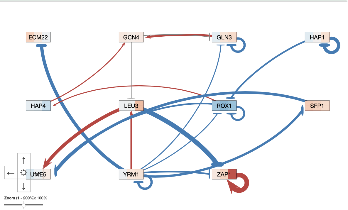
The GRNsight map produced using the output Excel worksheet showed 11 nodes and 21 edges.

The actual data was compared to the simulated data using GRNsight and revealed the following:

Wild type:

GCN4, ROX1, SFP1, and YRM1 had models that fit the data well. LEU3, and GLN 3 had less good fits, while ECM22, HAP4, UME6, ZAP1, and HAP1 had poor fits.

dgln3:

None of the genes had extremely good fits. SFP1, GLN3, ROX1, and LEU3 were moderate fits, while ECM22, HAP4, UME6, GCN4, YRM1, ZAP1, and HAP1 were poor fits.

dhap4

UME6 and HAP1 had close fits, SFP1 and GLN3 had moderate fits, while ECM22, HAP4, GCN4, LEU3, YRM1, ZAP1, and ROX1 had less good fits.

dzap1

YRM1, GLN3, and LEU3 had good fits. GCN4 and ROX1 had moderate fits, and ECM22, HAP4, UME6, ZAP1, HAP1, and SFP1 had extremely poor fits. ECM22 stood out has having the most poor fit.

GRNsight Model Data

Table 1. Number of incoming arrows to each node, ANOVA Benjamini & Hochberg corrected p-values, and gene expression based on the heat map presented at each gene's node. The GRNsight model used can be seen in Figure 1.

GRNsight Gene Network Model

Figure 1. GRNsight map developed using the Excel output file. The top and bottom data sets were set to "wt_log2_expression" and the average replicate values were used.

Parameter Graphs

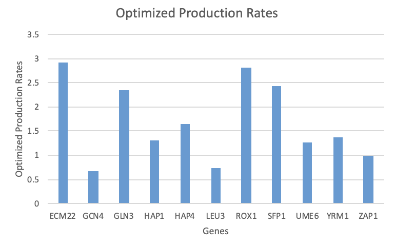
Figure 1. Optimized production rates for each gene as given in the Excel output workbook.

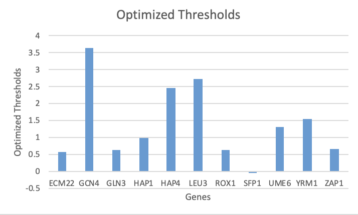
Figure 2. Optimized thresholds for each gene as given in the Excel output workbook.

Overall, there does not seem to be anything about these parameters that correlates to the goodness of fit found when analyzing the individual expression plots.

Data and Files

Excel output workbook and GRNsight and MATLAB results: linked here

In silico experiment files and results: linked here

Final Powerpoint presentation: linked here

Future Direction

For an upcoming in silico experiment, my homework partner Sahil and I decided to see what would happen if we didn't delete the nodes that weren't connected to anything from the "network" worksheet. The genes ARR1 and SMP1 were deleted from the original network (Week 4/5) because they appeared to be floating when input into GRNsight. However I would like to see if keeping these would impact the current findings, as the decision to delete these was based only on their appearance on GRNsight. I do not actually know for fact how insignificant these are to the network.

UPDATE (3/7/2019): After guidance from Dr. Dahlquist and Dr. Fitzpatrick in class on 3/7, it was decided that the in silico experiment described above may not produce any interesting findings. After discussing and analyzing the current gene map with Dr. Dahlquist, a new in silico experiment was proposed. Since the only grey lines in the map are coming out of GCN4, it may be interesting to see if deleting these relationships would create an impact. The "network" sheet in the GRNmap input Excel file was edited so that the two "1"s in the GCN4 column were set to "0". This new file was then run and the results were saved in the class Box folder as a "wt_in_silico" folder (linked in "Data and Files" section).

Conclusion

After analyzing the models created from the previous weeks using the individual expression plots and GRNsight, the goodness of fit of the outcome models to the data was evaluated. The LSE:minLSE ratio was determined to be 1.5738, and the individual expression plots showed that some genes had better fits than others. The line of dhap4 consistently did not match the data points, and all the lines in GCN4 were off from the data. However these findings could be skewed due to the fact that the location of some lines is unknown. In some of the plots, only two lines were visible, making it impossible to know which lines the remaining ones were behind. Overall, these findings did not seem to correlate to any patterns in the optimized production rates or threshold parameters. Lastly, the future in silico experiment chosen was to delete the relationship that GCN4 has with both GLN3 and LEU3 due to these being the only grey lines on the gene map.

Acknowledgments

I worked with my homework partner, Sahil. We texted a few times on 3/6 to decide which change to make for our in silico experiment. We also met for about 3 hours on Wednesday 3/20 to work on the Powerpoint presentation and communicated through text that day to finalize and polish it.

I also used Dr. Dahlquist and Dr. Fitzpatrick's help in class when we started the assignment on 3/5.

Except for what is noted above, this individual journal entry was completed by me and not copied from another source. Angela C Abarquez (talk) 21:12, 6 March 2019 (PST)

References

The Week 7 Assignment was used to create this journal entry. Specifically, the "Analyzing Results of First Model Run" and "Tweaking the Model and Analyzing Results" sections were used to describe the methods.

Dahlquist, K. & Fitpatrick, B. (2019). "BIOL388/S19: Week 7" Biomathematical Modeling, Loyola Marymount University. Accessed from:Week 7 https://openwetware.org/wiki/BIOL388/S19:Week_7 Week 7.