Alison S King Week 11

Purpose

The purpose of this assignment is to simulate a chemostat experiment and model the conservation of biomass and nutrient mass within this experiment. We will create this model by coming up with a set of representative differential equations and using MATLAB to create plots that compare the chemostat outcomes to the steady state outcomes.

Workflow and Results

Use the MATLAB files chemostat_script.m and chemostat_dynamics.m to simulate a chemostat and compare the computations to a steady state outcome. You will find those codes in the zipfile here

1. Use the parameter values q = 0.10 (1/hr), u = 5 (g/L), E=1.5, r=0.8 (1/hr), K = 8 (g). Using the formulae in the document (linked above), what are the steady states of cell biomass and nutrient mass?
   • • Steady-state of biomass: 2.5714 g
     • Steady-state of nutrient mass: 1.1429 g
2. Assuming a 2 liter chemostat, what are the steady state concentrations of cells and nutrient?
   • • Steady-state concentration of cells: 1.2857 g/L
     • Steady-state concentration of nutrients: 0.57145 g/L
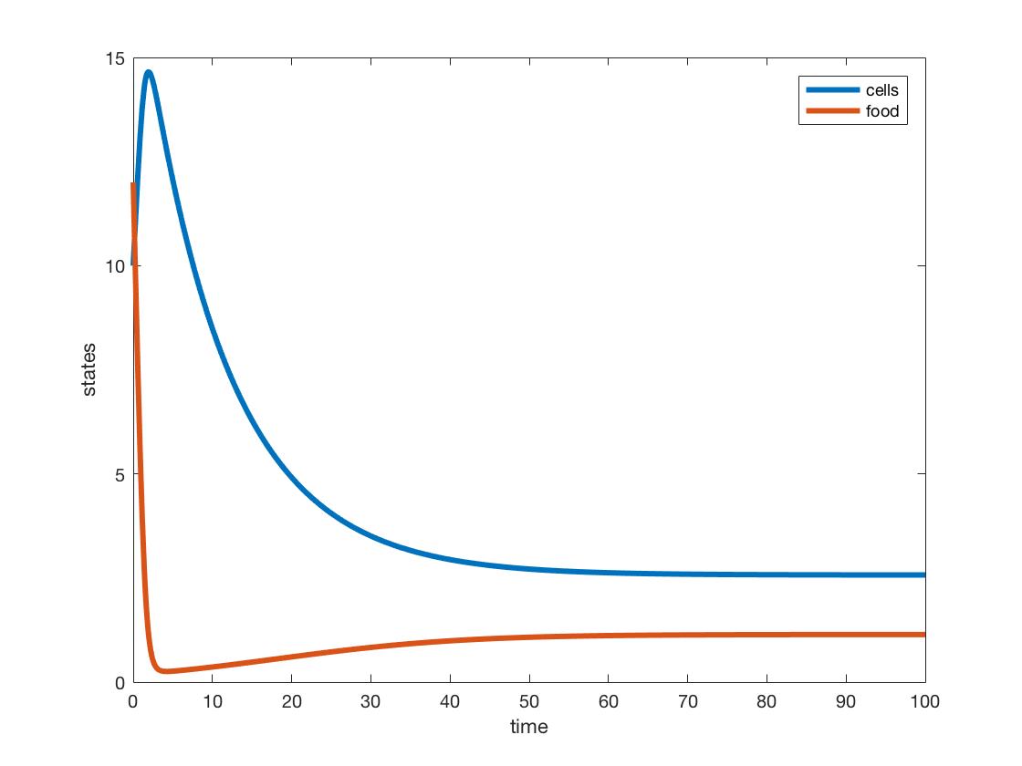
3. Simulate the system dynamics using the MATLAB files and the parameters of (1).
   • Do the graphs show the system going to steady state?
     • Yes.
   • Do the steady states match your (1) calculations?
     • Yes, when accounting for rounding error.
   • Be sure to save the graphs and upload them to your journal.
     • See Data and Files section below.
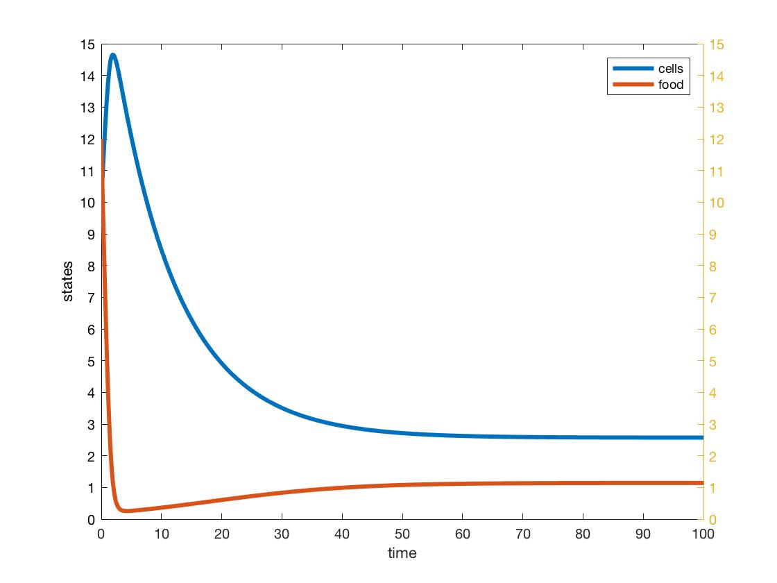
   • BONUS: can you get two y-axes, with the second one to the right of the picture like in the journal articles you’ve read?
     • See Data and Files section below.

Scientific Conclusion

By simulating a chemostat experiment, we were able to study the conservation of biomass and nutrient mass within the system. We modeled this conservation by using representative differential equations that describe the change of mass over time. By setting each differential equation equal to zero, we can find the steady state for each variable. Given our initial conditions and parameters, we ran the model in MATLAB and found that biomass reaches a steady state at 2.5714 g and nutrient mass reaches a steady state at 1.1429 g. The plot shows that nutrients initially turn into biomass before both variables reach their steady states. Our MATLAB model would allow us to rerun this experiment again with different parameters and initial conditions and compare the resulting plots.

Data and Files

Bonus Plot:

Acknowledgments

I would like to thank my partner, Angela, who I texted with about this week's assignment.

Except for what is noted above, this individual journal entry was completed by me and not copied from another source.

Alison S King (talk) 15:50, 10 April 2019 (PDT)

References

Loyola Marymount University (10 April 2019) BIOL388/S19:Week_11. Retrieved from https://openwetware.org/wiki/BIOL388/S19:Week_11 on 10 April 2019.

Links

Alison S King

Class Page: BIOL388/S19

Assignment Pages:

• Week 1
• Week 2
• Week 3
• Week 4
• Week 5
• Week 6
• Week 7
• Week 8
• Week 9
• Week 10
• Week 11
• Week 12
• Week 14/15

Shared Journals:

• Class Journal Week 1
• Class Journal Week 2
• Class Journal Week 3
• Class Journal Week 4
• Class Journal Week 5
• Class Journal Week 6
• Class Journal Week 7
• Class Journal Week 8
• Class Journal Week 9
• Class Journal Week 10
• Class Journal Week 11
• Class Journal Week 12
• Class Journal Week 14/15

Individual Journals:

• Alison S King Week 2
• Alison S King Week 3
• Alison S King Week 4/5
• Alison S King Week 6
• Alison S King Week 7
• Alison S King Week 8
• Alison S King Week 9
• Alison S King Week 10
• Alison S King Week 11
• Alison S King Week 12
• Alison S King Week 14/15