Moneil5 Week 4

Helpful Links

Margaret J. ONeil

Assignment Pages:

• Week 1 Assignment
• Week 2 Assignment
• Week 3 Assignment
• Week 4 Assignment
• Week 5 Assignment
• Week 6 Assignment
• Week 7 Assignment
• Week 9 Assignment
• Week 10 Assignment
• Week 11 Assignment
• Week 12 Assignment
• Week 14/15 Assignment

Personal Journal Entries:

• Week 1
• Week 2
• Week 3
• Week 4
• Week 5
• Week 6
• Week 7
• Week 7 Re-visited
• Week 9
• Week 10
• Week 11
• Week 12
• Week 14/15

Shared Journal Entries:

• Week 1
• Week 2
• Week 3
• Week 4
• Week 5
• Week 6
• Week 7
• Week 9
• Week 10
• Week 11
• Week 12
• Week 14/15

Purpose

The purpose of this assignment is to model the growth rate of yeast in a chemostat reactor using MATLAB and the ter Schure (1995) paper.

Methods/WorkFlow

• Used Week 4 Assignment PDF as a guide for investigating growth in chemostat cultures
• Created the function 'chemostatdynamics.m'

function dx = chemostatdynamics(t,x)
global q u V k r 
dx = zeros(size(x));
dx(1) = (q*u) - (q*x(1)) - (x(2)*((V*x(1))/(x(1)+k)));
dx(2) = (-q*x(2)) + ((r*x(2))*((V*x(1))/(x(1)+k)));
end

• Created the script 'ChemostatdynamicsScript.m'

global q u V k r 
q = 2;
u = 3;
V = 10;
k = 50;
r = 5;
tt = 0:0.1:10;
x0= [1,2];
[t,x] = ode45('chemostatdynamics',tt,x0);
plot(t,x)
xlabel('time')
ylabel('abundance')
title('Population and food source over time')
legend('Population','Food')

Where q, u, V, k, and r are parameters and state variables that can be changed, and thus random reasonable values for these variables were input into the script initially

• Played with the different variables and constants to see how it affected the model and plots
• Added a linear mortality term (-dx(2)), to the function 'chemostatdynamics.m'

function dx = chemostatdynamics(t,x)
global q u V k r d
dx = zeros(size(x));
dx(1) = (q*u) - (q*x(1)) - (x(2)*((V*x(1))/(x(1)+k)));
dx(2) = -(q*x(2)) + ((r*x(2))*(V*x(1))/(x(1)+K)) - (d*x(2));
end

• Added the variable d to the script 'ChemostatdynamicsScript.m'

global q u V k r d
q = 3;
u = .5;
V = 10;
k = 100;
r = 5;
d = 3;
tt = 0:0.1:10;
x0= [1,2];
[t,x] = ode45('chemostatdynamics',tt,x0);
plot(t,x)
xlabel('time')
ylabel('abundance')
title('Population and food source over time')
legend('Population','Food')

• Played with the value set for d in addition to the other parameters and state variables to see how the model was affected by the changes.
• Added a second nutrient to the function 'chemostatdynamics.m' which was required for growth of the population

function dx = chemostatdynamics(t,x)
global q u V k r d
dx = zeros(size(x));
dx(1) = (q*u) - (q*x(1)) - (x(2)*((V*x(1))/(x(1)+k)));
dx(2) = -(q*x(2)) + ((r*x(2))*(V*x(1))/(x(1)+k)) - (d*x(2));
dx(3) = (q*u) - (q*x(3)) - (x(2))*((V*x(1)+x(3))/(x(1)+x(3)+k));
end

• Added a term to the script 'ChemostatdynamicsScript.m' so that the script could run the three plots at once, the population, and food source 1 and food source 2

global q u V k r d
q = 3;
u = .5;
V = 10;
k = 100;
r = 5;
d  = 3;
tt = 0:0.1:10;
x0= [12,20,3];
[t,x] = ode45('chemostatdynamics',tt,x0);
plot(t,x)
xlabel('time')
ylabel('abundance')
title('Population and food source over time')
legend('Population','Food Source 1','Food Source 2')

• Played with variables and parameters to see how the model was affected by the value changes

Results

1. Consider the nutrient/cell population model...

   The differential equations being used are:

   dc/dt = qu - qc -yV_max(c/(K+c))

   dy/dt = yrV_max(c/(K+c)) - qy

   • The state variables are the nutrient concentration, c, and the population of yeast, y
   • The parameters are dilution rate, q, the feed concentration, u, the maximum volume, V_max and the growth rate r
   • The model is found to be at equilibrium when (c,y) = (u,0)

   The following are plots that demonstrate different nutrient levels, cell population size and constants

   Error creating thumbnail: Unable to save thumbnail to destination

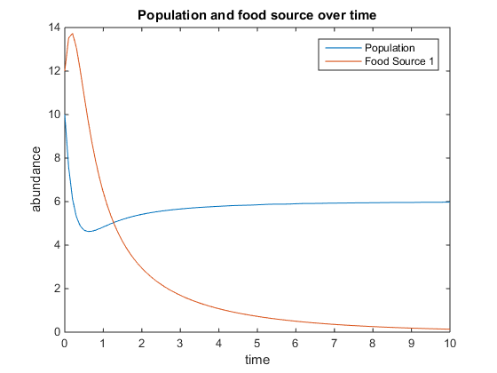
   Figure 1. Shows model using the following parameters:q = 4; u = 6; V = 10; k = 75; r = 5; and x0= [10, 12]

   Error creating thumbnail: Unable to save thumbnail to destination

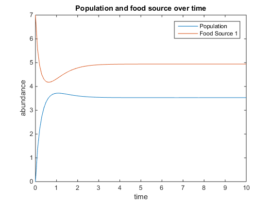
   Figure 2. Shows model using the following parameters:q = 3; u = 6; V = 10; k = 20; r = 2; and x0= [0, 7]

   Error creating thumbnail: Unable to save thumbnail to destination

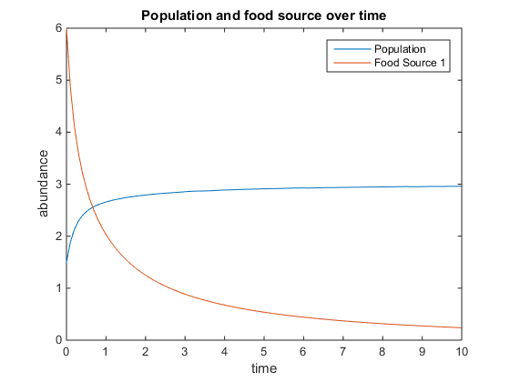
   Figure 3. Shows model using the following parameters:q = 5; u = 3; V = 20; k = 70; r = 6; and x0= [1.5, 6]

   Error creating thumbnail: Unable to save thumbnail to destination

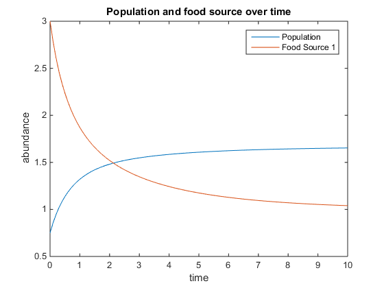
   Figure 4. Shows model using the following parameters:q = 1.5; u = 2; V = 5; k = 15; r = 3; and x0= [0.75, 3]

2. What changes if we return a mortality term to the population equation?

   • The model is still found to be at equilibrium when (c,y) = (u,0)
   • The following are plots that demonstrate different nutrient levels, cell population size and constants

   Error creating thumbnail: Unable to save thumbnail to destination

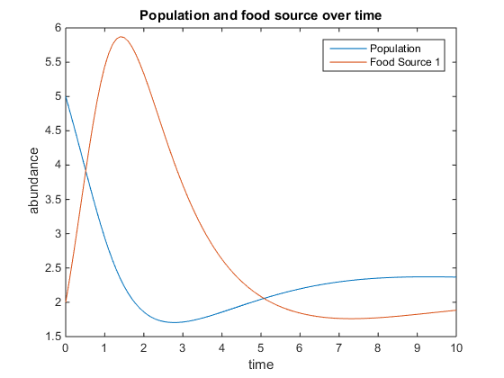
   Figure 5. Shows model where there is a linear mortality component added to the function. For this plot, q = .5; u = 3.5; V = 10; k = 75; r = 5; d = 1; and x0= [5, 2]

   Error creating thumbnail: Unable to save thumbnail to destination

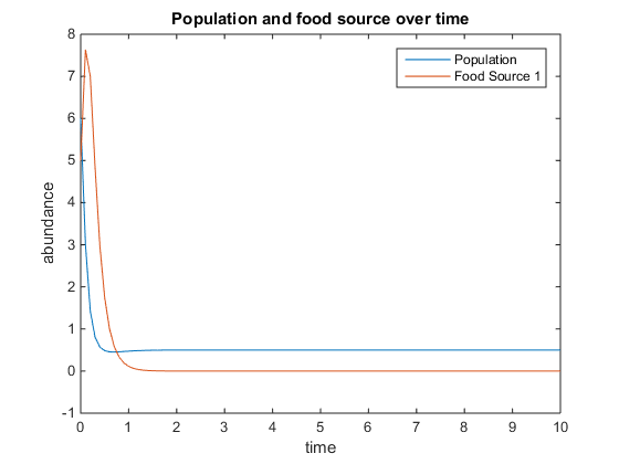
   Figure 6. Shows model where there is a linear mortality component added to the function. For this plot, q = 4; u = 0.5; V = 10; k = 15; r = 5; d = 3; and x0= [6, 5]

   Error creating thumbnail: Unable to save thumbnail to destination

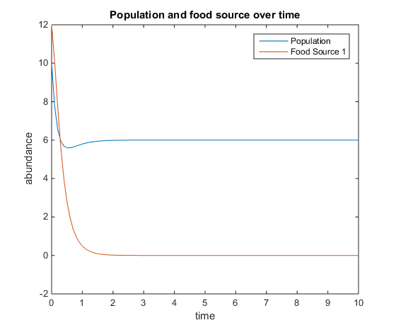
   Figure 7. Shows model where there is a linear mortality component added to the function. For this plot, q = 4; u = 6; V = 10; k = 75; r = 5; d = 3; and x0= [10, 12]

   Error creating thumbnail: Unable to save thumbnail to destination

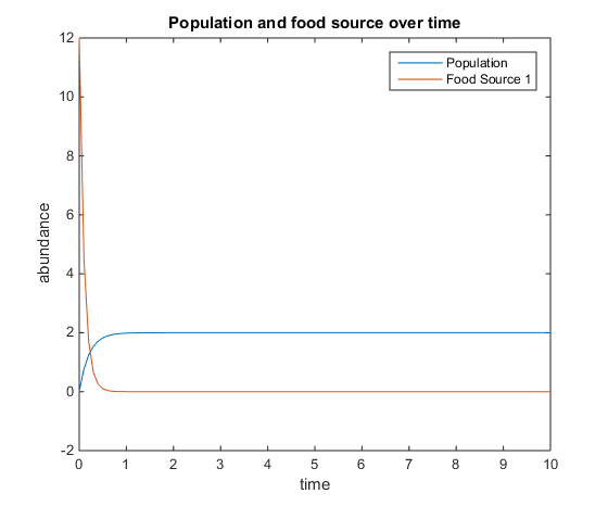
   Figure 8. Shows model where there is a linear mortality component added to the function. For this plot, q = 5; u = 2; V = 4; k = 75; r = 6; d = 5; and x0= [0, 12]

3. Create a model with two nutrients, both of which are required for the population to grow.

   Error creating thumbnail: Unable to save thumbnail to destination

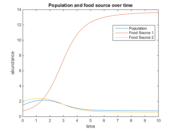
   Figure 9.This figure shows the relationships between nutrient concentration and population size when there are two available food sources

Conclusions

I successfully fulfilled the purpose of this assignment, which was to create 3 models of population growth in an open system (input and output) which was a chemostat. Through manipulating the state variables, parameters, and adding components to the models, it was found that across all models, there reaches a point where the nutrient concentration and yeast population become constant. This approaching of the constant value is due to the nature of the chemostat; the nutrient flow and food flow in was set at a fixed rate, and so was the output, which eventually lead to the plots reaching equilibrium. In manipulating the parameters and state variables, it was also found that nutrient concentration impacts yeast population, but so do dilution rates, mortality rates, volume of the chemostat, and additional food sources. Through these manipulations, it was found many factors in the chemostat system play a role in determining the growth rate of yeast.

Acknowledgements

• Based the function and script off of what Dr.Fitzpatrick showed us how to do in class
• Worked with the help of Lauren M. Kelly, Conor Keith, Cameron M. Rehmani Seraji, and Nika Vafadari in Seaver 120 to work on the MATLAB script and function
• Except for what is noted above, this individual journal entry was completed by me and not copied from another source.

Margaret J. Oneil 21:47, 8 February 2017 (EST)Italic text

References

• Dahlquist, Kam D. (2017) BIOL398-05/S17:Week 4. Retrieved fromWeek 4 Assignment PDF on February 8, 2017
• Dahlquist, Kam D. (2017) BIOL398-05/S17:Week 4. Retrieved fromWeek 4 Assignment on February 8, 2017