Lkelly9 Week 14/15
Navigation Links
- Lauren M. Kelly
- Assignment Page
- Individual Journal Entry
- Shared Journal Page
Purpose
Workflow/Methods
Dynamical Systems Modeling of your Gene Regulatory Network
For last week's assignment, you created a Microsoft Excel input workbook for the model. Now you are ready to run the model and analyze the results. The software we will use is called GRNmap, which stands for Gene Regulatory Network Modeling and Parameter Estimation. It is written in MATLAB and can be run from code or run as a stand-alone executable if you don't have MATLAB installed. However, it can only be run in Windows, not on Macs.
- To run GRNmap from code, you must have MATLAB R2014b installed on your computer.
- Download the GRNmap v1.4.4 code from the GRNmap Downloads page.
- Unzip the file. (Right-click, 7-zip > Extract here)
- Launch MATLAB R2014b.
- Open GRNmodel.m, which will be in the directory that you unzipped GRNmap-1.4.4 > matlab
- Click the Run button (green "play" arrow).
- You will be prompted to select your input workbook.
- You will see an optimization diagnostics graphic that shows the progress of the estimation.
- When the run is over, expression plots will display.
- Output .xlsx and .mat files will be saved in the same folder as your input folder, along with .jpg files containing the optimization diagnostic and individual expression plots. Save these files.
- Note that if you need to run GRNmap again, you should not use the same directory for the input file. Currently, GRNmap will overwrite previous output.
- Also note that you should run the model on the same computer if you want to compare model runs.
Analyzing the Modeling Results
In class on April 25, we will take a look at the modeling results and discuss how to analyze them. We will discuss:
- LSE/minLSE ratio
- MSE's and expression plots for individual genes in relation to their ANOVA p values
- Visualization of the weighted graph with GRNsight
- Making bar charts to give a graphical representation of the parameter values.
Based on these analyses, you will propose a some additional in silico experiments that you can do with the model. Some ideas are:
- For our initial runs, we estimated all three parameters w, P, and b.
- How do the modeling results change if P is instead fixed and w and b are estimated?
- How do the modeling results change if b is fixed and w and P are estimated?
- How do the modeling results change if P and b are fixed, and only w is estimated?
- For our initial runs, we included all three microarray datasets, wt, Δgln3, and Δhap4.
- What happens to the results if we base the estimation on just two strains (wt + one deletion strain)?
- What happens to the results if we base the estimation on just the wt strain data?
- When viewing the modeling results in GRNsight, you may determine that one or more genes in the network does not appear to be doing much.
- What happens to the modeling results if you delete this gene from the network and re-run the model (remember you will have to delete references to this gene in all worksheets of the input file).
Final Research Presentation
- You and your partner together will prepare a 20-30 minute PowerPoint presentation that will present the results of your final project. Please follow these guidelines when creating your presentation. You will need approximately 20-30 slides (1 slide per minute) for your presentation. You will be graded according to this rubric.
- Upload your slides to the OpenWetware wiki by the Week 14/15 journal assignment deadline (midnight on May 4). Each partner should have a link to the same PowerPoint file. You may make changes to your slides in advance of your presentation, but you will be graded on what you upload by the journal deadline.
- Your presentation will include the following:
- Title slide that gives the main take-home message as the title of your presentation, the authors, date, and venue (course number and title).
- Outline slide that is a summary of take-home messages of your talk (should mirror your conclusion slide)
- The body of your talk (more details below)
- Conclusion slide that mirrors your outline
- Future directions
- Acknowledgments
- References
Introduction & Background
The introduction gives the background information necessary to understand the motivation for your project and your research results. The introduction should be in the form of a logical argument that "funnels" from broad to narrow. Include the following:
- States importance of the problem
- Why are we studying gene regulation and cold shock?
- States what is known about the problem
- Introduce the DNA microarray experiment that was performed.
- States what is unknown about the problem
- Little is known about which transcription factors regulate the early response to cold shock
- States clues that suggest how to approach the unknown
- Each of the journal club articles that you all presented has a piece of the puzzle that motivates this project
- States the question the project is trying to address
- Using the model to estimate the relative contribution of each transcription factor to the regulation of gene expression
Methods
- Describe the entire workflow of this project using a flow chart diagram.
- Experimental design of the microarray experiment
- Statistical analysis of the microarray data
- Clustering and GO term analysis
- Finding candidate transcription factors with YEASTRACT
- Generating and paring down the adjacency matrix
- The differential equation and least squares equation that were used for performing the initial estimation
- Creating the input workbook and how that relates to those equations
- Analyzing the modeling results
- Additional in silico modeling experiments
Results & Discussion
- Table of ANOVA results from the Week 11 Assignment, discussing the interpretation of the p values.
- From the STEM analyis, include as figures the overall results (the screenshot showing all of the clusters) and then focus on the ones you interpreted for your journal assignment.
- Include a table showing the GO results for that cluster (just the narrowed down list of terms that you have interpreted).
- Discuss what the p values for the cluster and for the GO term list mean.
- Discuss the biological interpretation of your GO terms.
- Include a table that lists the transcription factors that you and your partner are working with and their enrichment p value from YEASTRACT (from the Week 12 Assignment). Include just the transcription factors that made it into your final networks.
- Describe how and why you and your partner chose these transcription factors for your networks.
- Include a figure of the unweighted networks visualized with GRNsight.
- Modeling results (from the current assignment), including the LSE/minLSE ratio for each model run. Include the following parameter bar charts
- Optimized weight parameters (w)
- Optimized production rates (P)
- Optimized threshold b parameters
- Show the individual expression plots for each transcription factor for one of the initial runs, with the MSE and ANOVA values for each gene superimposed. You will want to organize these so that they can be compared easily. For the subsequent runs, compare plots for "interesting" genes with each other.
- Show the GRNsight visualization of the weighted networks, making sure that the genes are placed in the same relative location as each other an as the unweighted network figure.
- Interpret the results of the model simulation.
- Examine the graphs that were output by each of the runs. Which genes in the model have the closest fit between the model data and actual data? Which genes have the worst fit between the model and actual data? Why do you think that is? (Hint: how many inputs do these genes have?) How does this help you to interpret the microarray data?
- Which genes showed the largest dynamics over the timecourse? In other words, which genes had a log fold change that is different than zero at one or more timepoints. The p values from the Week 11 ANOVA analysis are informative here. Does this seem to have an effect on the goodness of fit (see question above)?
- Which genes showed differences in dynamics between the wild type and the other strain your group is using? Does the model adequately capture these differences? Given the connections in your network (see the visualization in GRNsight), does this make sense? Why or why not?
- Examine the bar charts comparing the weights and production rates between the two runs. Were there any major differences between the runs? Why do you think that was? Given the connections in your network (see the visualization in GRNsight), does this make sense? Why or why not?
- Finally, based on the results of your entire project, which transcription factors are most likely to regulate the cold shock response and why?
- How do you interpret the results of the additional in silico experiments you performed with the model in light of the above?
- Relate the results of your project to the paper you presented for journal club in Week 10
- What future directions would you take if you were to continue this project?
Results
Analyzing the Modeling Results
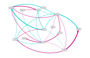
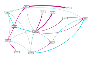
- In order to further investigate the network, I started with the original 14 nodes and 33 edges network and did 3 different runs.
- Deleted HMS1 (13 nodes, 27 edges)
- Deleted GLN3 (13 nodes, 32 edges)
- Deleted SPT23 (13 nodes, 23 edges)
- GRNsight visualizations for each of these network runs are shown on the right.


Conclusion
- SPT23 and GLN3 appear to be important in regulating the cold shock response
- While GLN3 was not significant according to YEASTRACT, the production rates/optimized weights bar charts and the GRNsight visualizations indicate that removing GLN3 changes the network.
- SPT23 consistently regulated many of the transcription factors and was a central part of the GRNsight visualization
- The deletion of SPT23 changed various things about the network
- Future studies would include why GLN3 appears to have an effect despite the insignificant p-value from YEASTRACT and continuing to manipulate the model to see if other transcription factors play an important role in cold shock response
Acknowledgments
- Worked with Cameron M. Rehmani Seraji in Seaver 120 on May 3rd to put together the presentation.
- Methods were copied from the Week 14/15 assignment page.
- Except for what is noted above, this individual journal entry was completed by me and not copied from another source.
Lauren M. Kelly 23:15, 3 May 2017 (EDT)
References
- Dahlquist, Kam D. (2017) BIOL398-05/S17:Week 14/15. Retrieved from http://www.openwetware.org/wiki/BIOL398-05/S17:Week_14/5 on 3 May 2017.
- Tai, S. L., Daran-Lapujade, P., Walsh, M. C., Pronk, J. T., & Daran, J. M. (2007). Acclimation of Saccharomyces cerevisiae to low temperature: a chemostat-based transcriptome analysis. Molecular biology of the cell, 18(12), 5100-5112.
