Understanding Mathematic Modeling in Response to Pandemics

Purpose

To identify the influences of various disease traits on infection dynamics.

Combined Methods and Results

Preparatory work

The following sources were read or watched for background on disease modeling:
After watching The role of applied math in real-time pandemic response: How basic disease models work, two questions were recorded.
1. If Rate 2 (Rate of Recovery) varies between individuals, does Rate 2 reflect the mean recovery rate?
2. How do we account for if immunity/vaccination is not permanent?
After reading the article The SIR Model: Using Math to Save the World: Math Can Predict the Spread of Infectious Diseases, four questions were answered regarding the model graph in this article.
1. What happens if initial I = 0?
  - If initial I=0, then no infections will take place. Therefore, I will remain at zero.
2. What does it mean that red line increases so rapidly?
  - A rapid increase in the red line indicates a high Rate 1 or rate of infection.
3. What does it mean that green line also rises rapidly, but not as rapidly?
  - A rapid increase in I (but not as rapid as red) means that recovery rate (Rate 2) is also relatively high. Unless a disease takes 0 days to reach recovery (or death), the green line will always have a lower slope than red.
4. What does it mean that the green line reaches nearly to 1,000?
  - This means nearly all of the population has recovered. The slight discrepancy from exact 1,000 accounts for deaths.
The Epidemix modeling website was used for the following steps.
1. Start button was pressed
2. Deterministic model type was chosen in order to see influences of fixed parameters. In cases such as COVID-19, infection and recovery rates can be found. Using these fixed rates, one can project disease status to inform social policy. Homogenous mixing model type chosen for initial models. Heterogenous models shown in later parameter adjustments for comparative purposes of how differently models can look when considering different contact rates.
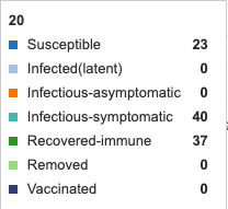
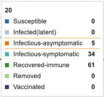
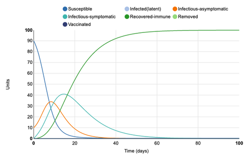
3. Initial model graph was screenshot for reference and comparison to parameter adjustments. Individual infection state data provided at day 20 for comparative purposes.
4. Various parameters were adjusted and compared to initial graph

Initial Graph

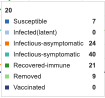
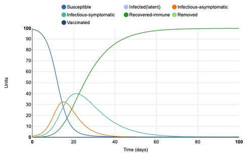
Figure 1: Initial conditions of Epidemix Deterministic Homogenous Model. Individual infection state data provided at day 20 for comparative purposes.

E and I(a) infection states added

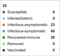
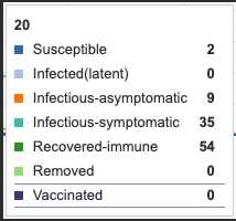
E (Extinct) and I(a) (infectious-asymptomatic) infection states were added to the model. This adds a new line to the visual. The symptomatic curve is shifted about two days to the right. This may be accounting for a two day asymptomatic period. It can also be seen that infection rate (the rate at which units move out of the S susceptible state) is increased. The Blue susceptible line is dropping more rapidly. At day 20, only 8 remain in the S state whereas before asymptomatic infections came in, day 20 had 23 units in S state. Extinct (E) state has no influence as parameter has not yet been defined.

Figure 2: E (extinct) and I(a) (infectious-asymtomatic) infection states added to model. Individual infection state data provided at day 20 for comparative purposes.

Latency Period of 14 Days

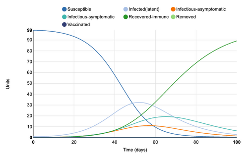
Adding a latency period of 14 days greatly extends the S->I transition. This 14 day period is where a unit is infected but not infectious. 100% of units have still been infected by day 100 but the infected period has been lengthened. The maximum amount of infectious, symptomatic individuals at a single point in time is 20 units, however, the period in which units are symptomatic has been lengthened to go beyond 100 days. By adding a latency period to a disease, the curve is effectually "flattened".

Figure 3: Latency period of 14 days added to model. Individual infection state data provided at day 20 for comparative purposes.

Asymptomatic Period of 14 Days

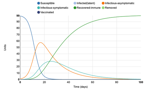
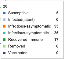
Asymptomatic period was extended from 5 days to 14 days. This produces much more rapid increase in infectious asymptomatic cases. The peak asymptomatic cases increases from 32 to 58. The peak for infectious-symptomatic, however, decreases from 40 units to 29 units and the period in which units are symptomatic is extended. So, once again, the curve is effectually flattened

Figure 4: Asymptomatic period of 14 days added to model. Individual infection state data provided at day 20 for comparative purposes.

Symptomatic Period of 20 Days

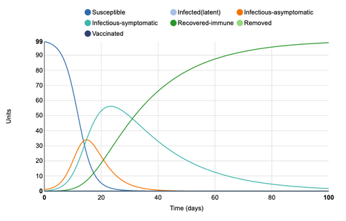
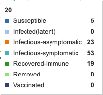
When symptomatic period is extended from 10 to 20 days, the peak of symptomatic cases increases from 40 units to 55 units.

Figure 5: Symptomatic period of 20 days added to model. Individual infection state data provided at day 20 for comparative purposes.

Effective Contact Rate Increased to 1/day

The effective contact rate was increased from 0.4 per day to 1 per day. The S pool decreases much more rapidly. The infectious asymptomatic peak increases from 32 to 55. The infectious symptomatic peak also increases from 40 to 49. These peaks also happen earlier as infection rate has increased. These two curves are also shortened in duration. However, the day of full population recovery has remained nearly the same, only shifting two days earlier.

Figure 6: Effective contact rate increased from 0.4/day to 1/day. Individual infection state data provided at day 20 for comparative purposes.

Initial Cases Increased to 10 units

When the initial cases were increased to 10, the only change is that all events are shifted to happen about 10 days earlier. Peaks remain the same and so do durations of infectious units both symptomatic and asymptomatic.

Figure 7: Initial cases increased to 10. Individual infection state data provided at day 20 for comparative purposes.

Death Rate Increased to 0.3

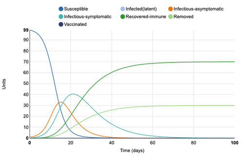
When rate of removal is increased from 0 to 0.3 (which is fairly high considering this is 30%), nothing changes except 30% of the population that would have ended up in the Recovered category are now included in the Extinct category. Infection rates do not change as death serves the same function as recovery in a disease model.

Figure 8: Death rate increased to 30%. Individual infection state data provided at day 20 for comparative purposes.

Density Dependent Mode of Transmission

Mode of transmission was changed from frequency-dependent to density-dependent. No changes.

Figure 9: Mode of transmission changed from frequency dependent to density dependent. Individual infection state data provided at day 20 for comparative purposes.

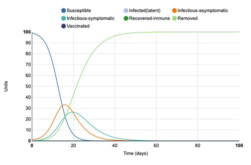
Culling for 5 Days

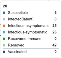
When culling treatment was added for 5 days, the symptomatic-infectious category decreased its peak from 40 to 25. These units were effectively removed from the infectious pool and therefore added into the removed (however, not immune) category.

Figure 10: Culling for 5 days added as a treatment. Individual infection state data provided at day 20 for comparative purposes.

Vaccination

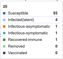
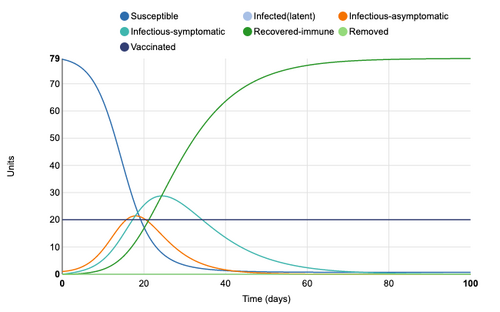
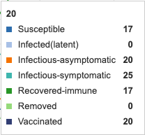
Vaccination parameter was set to vaccinate 20% of the population. 20 units were removed from susceptible pool and entire model was reduced in magnitude by 20%. Recovery took place on a similar time scale, ending on the same day.

Figure 11: Vaccination was added for 20% of population. Individual infection state data provided at day 20 for comparative purposes.

Giordano et al.

Figure 1 of Giordano et al (2020) was used to answer two questions from BIOL368/F20:Week_2
1. How did the authors modify the simple SIR model to take into account features of the COVID-19 pandemic?
  - Infected now means infected, asymptomatic, and undetected. The original "Infected" state has also expanded into the states of Diagnosed (asymptomatic and detected), Ailing (symptomatic, undetected), Recognized (symptomatic, detected), and Threatened (symptomatic, detected, and at risk of death). The rates between each infection state are also independent. All of these factors have created a model more accurate for the COVID-19 pandemic at hand(Giordano et al. 2020).
2. What public health policy implications does their model have?
  - Social distancing must be adhered to. Lockdown can only be safely lifted if testing is widespread enough to cover the Infected and Ailing populations. Population wide testing is essential to move individuals from I and A to D and R where quarantining can then take place and effectively put those individuals into the removed pool (Giordano et al. 2020).

Web Comic

This comic was reviewed for purposes of humor
- If a physicist were using Giordano's (2020) model, it can be assumed that alpha, beta, gamma, and delta were extremely underestimated based upon the physicists lack of knowledge as to the magnitude of person to person contact at college social gatherings.

Conclusion

Various disease parameters have various influences on disease spread dynamics. These influences include: extending or reducing the period of infection, increasing or decreasing the maximum infected at a given time, and alterations in the balance between symptomatic and asymptomatic units. These disease traits and subsequently modeled outcomes should be taken into consideration when producing public policy in response to each unique disease.

References

Giordano, G., Blanchini, F., Bruno, R., Colaneri, P., Di Filippo, A., Di Matteo, A., & Colaneri, M. (2020). Modelling the COVID-19 epidemic and implementation of population-wide interventions in Italy. Nature Medicine, 1-6.
NIMBioS (1 April 2020). The role of applied math in real-time pandemic response: How basic disease models work (Video). Retrieved from [1]
Wheeling Jesuit University. SIR Model (Web Article). Retrieved from [2]
BIOL368/F20:Week_2

Acknowledgements

Schnell, S. (2015). Ten Simple Rules for a Computational Biologist’s Laboratory Notebook. PLoS Comput Biol, 11(9), e1004385. Was referenced for assistance on journal structure.
Syntax from BIOL368/F20:Week_1 was copied and edited for image attachment.
Questions from BIOL368/F20:Week_2 were copied and pasted into Methods section and modified for syntax purposes.
Media Wiki Help was used to help format images
Consulted with Nida Patel on parameter adjustments, acknowledgement contents, and explanation format.
Except for what is noted above, this individual journal entry was completed by me and not copied from another source.

Ian R. Wright (talk) 21:55, 16 September 2020 (PDT)