JT Correy Journal Week 2
Journal Week 2
Purpose
This purpose of the week two lab is analyze various SIR models of diseases and identify how they relate to COVID-19 in order to understand models of COVID-19.
Tasks
This week, you will begin documenting your workflow in your individual journal entry. Refer to Schnell et al. (2015) for rationale and guidelines that professional computational biologists use. You need to describe what you did in enough detail that someone else can reproduce it using only your documentation. You may copy and modify these instructions, making sure to Acknowledge this properly and cite this page in your References section.
- Watch the video: The role of applied math in real-time pandemic response: How basic disease models work
- Record two questions that you have after watching the video.
- Towards the end of the video, she speaks about the more complicated equations for her model. How are the COVID-19 equations more complicated than the base one, and what do those complexities calculate?
- What are the rates of infection and recovery for COVID? I know there is still a huge lack of data, but I am very interested to see what the actually rates are when everything gets more organized.
- Record two questions that you have after watching the video.
- Read the information on this website.
- Look at the graphs and make sure you understand how to interpret them by answering the questions:
- What happens if initial I = 0?
- In the equation I represents the number of infected people, so of the initial I = 0 then there will be no spread of the disease because no one will have it in the first place.
- What does it mean that red line increases so rapidly?
- The rapid increase of the red line means that the disease is spread between people very easily. The steeper the slope, the more people become infected, thus the faster the disease can spread.
- What does it mean that green line also rises rapidly, but not as rapidly?
- The green line represents the recovered population. The green line's semi-rapid increase means that many people recover in a fairly quick time period. The fact that it does not increase as fast as the red line means that people are not recovering as quickly as they get infected.
- What does it mean that the green line reaches nearly to 1,000?
- The green line almost reaching 1,000 means that almost everyone has recovered. However, given that there are no more infections, we can attribute the 20 people not recovered to deaths.
- What happens if initial I = 0?
- Look at the graphs and make sure you understand how to interpret them by answering the questions:
- You will now explore an online, interactive SIR model, Epidemix.
- Go to the website and click the "Start" button in the middle of the page.
- Select the type of model you will explore from the drop-down menu on the upper-left side of the page. Explain why you made that choice.
- I chose the Stochastic Homogeneous Mixing-ASF because COVID-19 is thought to have come from mammals and the Swine Flu came from pigs so pig to human disease jumps are certainly possible. My partner also chose this model so we could compare.
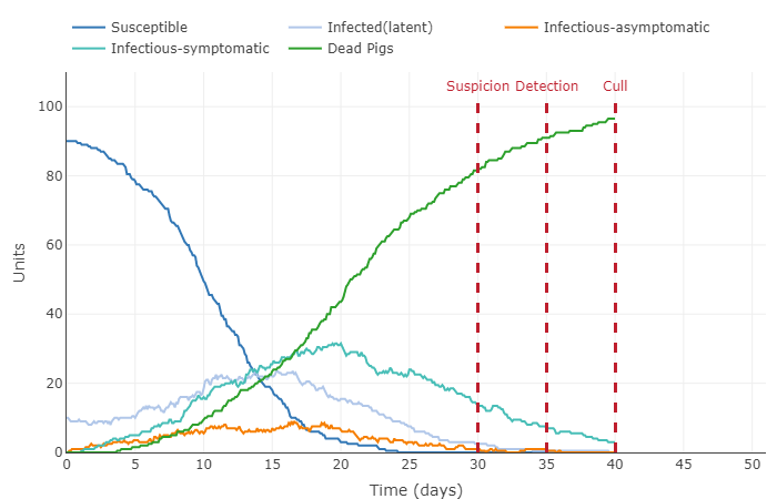
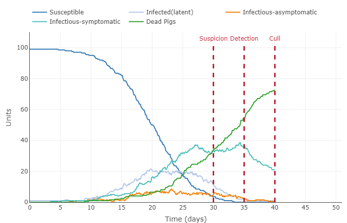
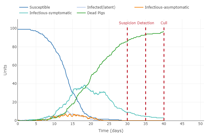
- Take a screenshot of the initial plot that is shown on the page and display it on your individual journal page (remember, this will be a 2-step process to upload the image file and then display it on your page).

- This graph shows the pig population getting infected fairly quickly. 100 percent of pigs were infected around the 37th day, this the majority of those pigs dying before the culling on day 40. All the latent, asymptomatic, and symptomatic infections percentages were below 20 percent of the total population.
- Now you will explore the model by changing the parameters and seeing what happens to the graph.
- Choose one parameter to change at a time. It will be helpful to make "extreme" changes so that you are sure to see a difference. You and your partner can collaborate and make different changes to the parameters and compare your results.
- Make the change and display the plot on the Epidemix website.
- Take a screenshot of the plot and display it on your individual journal page.
- Describe in words what happened to the plot, thus interpreting the effect of the parameter change in the model.
- Repeat this process 9 more times so that in the end, you will have 11 total screenshots. The initial conditions and 10 cases where you changed one parameter.
- Now you will explore the model by changing the parameters and seeing what happens to the graph.
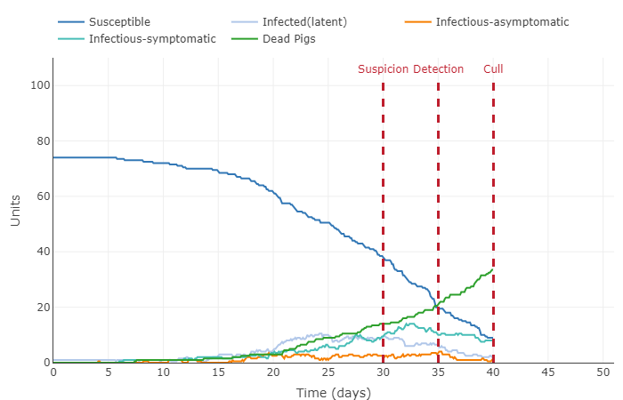
- Increased starting infected rate by 10%
- This graph is very similar to the first, but has a much steeper curve for the susceptible group. By with a larger infected population, the disease spreads much faster. There are also many more pigs in the latent, asymptomatic, and symptomatic infections.
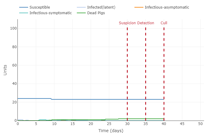
- Decreased number of contacts from 0.62 to 0.1
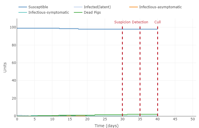
- This graph is quite different from the original. When the pigs are isolated from each other the disease has almost no ability to spread. With this parameter only 2 percent of the population was ever infected.
- Increased number of contacts from 0.62 to 1
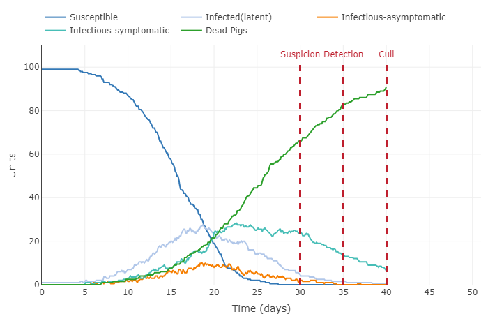
- This graph is similar to the graph with a larger starting population. The more contacts by the pigs causes the disease to be spread much more quickly. All the pigs have been infected before day 30, which is almost as fast as starting out with ten times in the infected population.
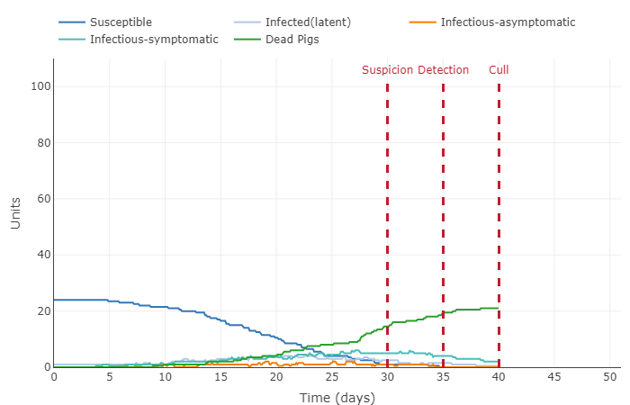
- Infectious period changed from 6.5 to 1
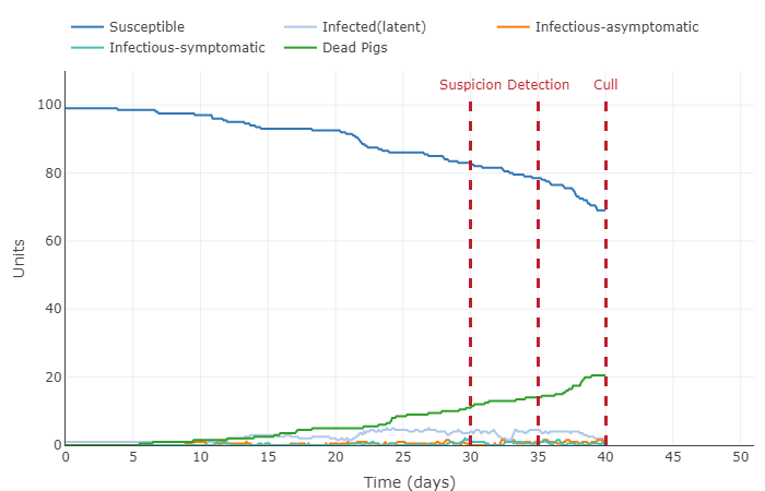
- This graph displays a new variation. There is a much flatter cure of susceptible pigs. The decreased infectious period means that at any given time there will be less pigs infected, thus there is significantly slower transmission of the disease.
- Infectious period changed from 6.5 to 10
- This graph is pretty similar to the increased contact graph. As the pigs have the disease longer they are going to come into contact with more pigs over the time they are infected, and thus the disease spreads quickly with all the pigs being infected by day 35.
- Added a vaccine that is 25% effective
- This graph is essentially the same as the orginaly graph, but with a reduced maximum of susceptible pigs. The 25% of immune pigs are not susceptible so they decrease the rate that the disease spreads to an almost liner rate.
- Increased vaccine success rate to 75%
- This graph shows a very interesting concept: herd immunity. Because a significant amount of the population (75%) is immune to the disease, the infected pigs barely come into contact with a susceptible pig. This the disease cannot spread quickly and eventually dissipates (until the next generation that is not immune comes along).
- Increased number of contacts to 2 and kept the vaccine success rate at 75%
- This graph shows that even though the vaccine has been given to three fourths of the population, the lack of isolation of the infected pigs allows all the susceptible pigs to still be put in danger. Of course the disease does not infect the immune group, but the rest of the pigs become infected.
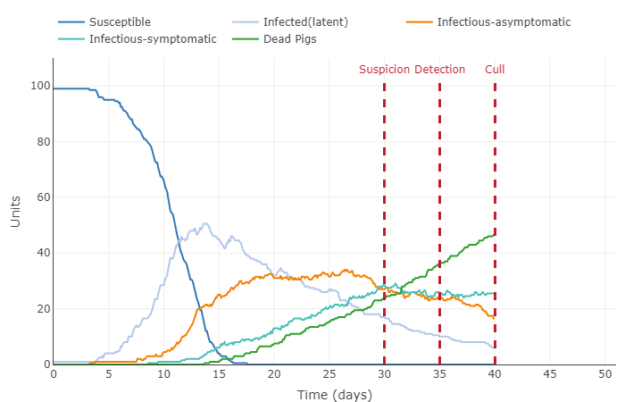
- Decreased length of asymptomatic and latent infections to last 1 day
- This graph shows that it is primarily the symptomatic pigs that transmit the disease. There is still a significant amount of latent pigs. This alteration did not make that much of a difference because the infection period for the symptomatic pigs is still so high.
- Increased all infection periods to 10 days and increased contact rate to 4
- This graph shows an extremely rapid infection rate. All the pigs are infected by day 17 because the contract rate is so high and so many of the pigs have the disease at any given point (due to the long infection periods).


Look at Figure 1 of the Giordano et al. (2020) article.
- How did the authors modify the simple SIR model to take into account features of the COVID-19 pandemic?
- The authors added more categories other than the normal susceptible, recovered, and infected. They include options like diagnosed, threatened, and ailing, and recognized.
- What public health policy implications does their model have?
- This figure is likely much more useful to policy makers then the normal/basic model. This includes many more real-life options, like people who are sick but have note been tested. Thus this model is much more likely to be more accurate and provide more reliable data to the community.
Check your understanding: https://xkcd.com/2355/. Why is this comic funny? (Hint: hover your mouse over the graphic to see the extra joke in the tooltip.)
- The XKCD comic makes fun of physics majors not being invited to parties as much as other college students. This is really important think about when creating a COVID model. As was shown in the earlier graphs, more contacts lead to significantly more infected people.
Write your scientific conclusion: a summary statement of the main result of exercise/research. It should mirror the purpose. Length should be 2-3 sentences, up to a paragraph.
- This lab was very informative. The SIR model is a fantastic tool to analyze disease spreading and be able to manipulate different aspect of a disease or population. It is exceedingly applicable to the situation the world is now with COVID-19. The Model by Giordano et al was a well-modified SIR graph that presents a more realistic representation of how COVID-19 infects people. Models can and should be used to portray crucial information regarding diseases.
Acknowledgements
- Nathan Beshai
- Nathan And I were homework partners this week. We communicated mostly over text. We worked together on the SIR model manipulation and chose the same one so that we could compare. I also referenced his week 2 journal while I was creating mine.
- Dr. Dahlquist
- Dr. Dahlquist served as a coach for how to use OpenWetWare. She also instructed the class and provided us with the guiding homework document.
Jcorrey (talk) 19:40, 16 September 2020 (PDT)
- Except for what is noted above, this individual journal entry was completed by me and not copied from another source.
References
- OpenWetWare. (2020). BIOL368/F20:Week 2. Retrieved September 16, 2020, from https://openwetware.org/wiki/BIOL368/F20:Week_2
- OpenWetWare. (2020). User:Nathan R. Beshai. Retrieved September 16, 2020, from https://openwetware.org/wiki/User:Nathan_R._Beshai
- Video: The role of applied math in real-time pandemic response: How basic disease models work
- The SIR Model: Using Math to Save the World: Math Can Predict the Spread of Infectious Diseases
- Giordano, G., Blanchini, F., Bruno, R., Colaneri, P., Di Filippo, A., Di Matteo, A., & Colaneri, M. (2020). Modelling the COVID-19 epidemic and implementation of population-wide interventions in Italy. Nature Medicine, 1-6. DOI: 10.1038/s41591-020-0883-7
- Schnell, S. (2015). Ten Simple Rules for a Computational Biologist’s Laboratory Notebook. PLoS Comput Biol, 11(9), e1004385. DOI: 10.1371/journal.pcbi.1004385
JT Correy Template
Weekly Assignments
- Week 1 Assignment
- Week 2 Assignment
- Week 3 Assignment
- Week 4 Assignment
- Week 5 Assignment
- Week 6 Assignment
- Week 7 Assignment
- Week 8 Assignment
- Week 9 Assignment
- Week 10 Assignment
- Week 11 Assignment
- Week 12 Assignment
- Week 14 Assignment
Individual Journal Pages
- JT Correy
- JT Correy Journal Week 2
- JT Correy Journal Week 3
- JT Correy Journal Week 4
- JT Correy Journal Week 5
- JT Correy Journal Week 6
- JT Correy Journal Week 7
- CancerTracer Review
- JT Correy Journal Week 9
- JT Correy Journal Week 10
- JT Correy Journal Week 11
- JT Correy Journal Week 12
- JT Correy Journal Week 14
- The Mutants Week 14
Class Journal Pages
- BIOL368/F20:Class Journal Week 1
- BIOL368/F20:Class Journal Week 2
- BIOL368/F20:Class Journal Week 3
- BIOL368/F20:Class Journal Week 4
- BIOL368/F20:Class Journal Week 5
- BIOL368/F20:Class Journal Week 6
- BIOL368/F20:Class Journal Week 7
- BIOL368/F20:Class Journal Week 8
- BIOL368/F20:Class Journal Week 9
- BIOL368/F20:Class Journal Week 10
- BIOL368/F20:Class Journal Week 11
- BIOL368/F20:Class Journal Week 12
- BIOL368/F20:Class Journal Week 14
