Purpose

The purpose of this assignment is to develop a better understanding of exponential and logistic growth models by plotting the solution to the logistic growth ODE using Matlab.

Workflow

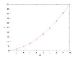
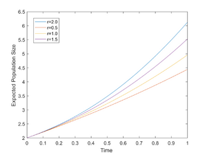
The data used in this exercise is available on the Week 2 assignment page, which is linked at the bottom of this page. Both part one and part two of the assignment were completed in Matlab. For the first exercise I opened a new script in Matlab and defined two vectors U and V. Where U=[1,2,3,...,10] ad V=U^2. I then plotted the two vectors with V on the x-axis and U on the y-axis. I then saved this plot as figure 1. The plot is available in the top right hand corner of this page titled "Figure 1." For part two, I opened a new script in Matlab then defined 4 variables K, y0, tspan, and r. Here K is the carrying capacity and is equal to 10, y0 is the initial population size and is equal to 2, tspan is the timespan which ranges from 0 to 1 in increments of 0.01, and r is the growth rate of the population which took on values 0.5,1,1.5, and 2. I then constructed the population growth ordinary differential equation solution we covered in class using Matlab's ODE45 function. I concluded the script by plotting the solutions with time on the x-axis and population size on the y-axis.

Figure 1 is a simple model for exponential population growth. Consider the U vector to be time and the V vector to be population size, then it is clear that population size grows expontentially as time increases. Figure 2 is a solution model to the logistic growth differential equation that was covered in class with varying growth rates. The model only covers a time span of one, so it is clear that the population is still in the exponential growth stage where resources are more abundant. You can see at time=1, the growth rate of the population is beginning to slow, which is consistent with the theory discussed in class. As time passes, resources become more scarce and reproduction rates begin to decline. Eventually, the differential equation will have a vertical asymptote at the carrying capacity K=10. This means the population, y, will eventually settle at ten.

I was able to construct simple models of logistic and exponential growth. These simple models allowed me to analyze population growth patterns and the factors that determine growth rates, namely carrying capacity. The model from part two shows that populations do in fact trend towards their carrying capacity over time. The model also shows that regardless of growth rate, the expected population value will always trend to K.

For this weeks assignment my homework partners were Cameron and Lauren, but I was unable to get in contact with my partners. I received the data and instructions for this weeks assignment from the Week 2 assignment page on our course Wiki page, which is linked at the bottom of this page. I also made use of the Matlab websites ODE45 help page to refresh my memory on how to properly execute the function. Except for what is noted above, this individual assignment was completed by me and not copied from any other source.

Conor Keith 02:37, 26 January 2017 (EST)

Assignment Pages:

Individual Journal Entries :

Shared Journal Pages:

References

BIOL398-05/S17:Week 2 (2016). In OpenWetWare. Retrieved January 22, 2016, from https://openwetware.org/wiki/BIOL398-05/S17:Week_2#This_Week.27s_Modeling_Exercise
Ode45. (n.d.). Retrieved January 23, 2017, from https://www.mathworks.com/help/matlab/ref/ode45.html