User:Nuri Purswani/Network/SyntheticDatasets

Algorithms for Biological Network Reconstruction from data

Home

Introduction

Synthetic Datasets

Methods

Results

Discussion

References

Synthetic Datasets

The observed output from gene expression profiling experiments depends on internal unmeasured states and external inputs, such as noise or external disturbances (Wu et al. 2004, Rangel et al. 2004, Kusalik et al. 2009). State space models are commonly used representations for simulation of gene expression experiments, as they take into account that the observed effects from the experiments can be fully described by the 'state' of unobserved effects. For examples where these models have been implemented in the simualation of gene expression see: Gonçalves et al. 2008, Alche-Buc et al. 2007, Beal et al. 2005, Rangel et al. 2004. The latter references also provide detailed derivations and alternative notations. Here we describe the state space form in continuous time, and its relevance in describing biological gene-gene interactions.

In Silico Test Networks

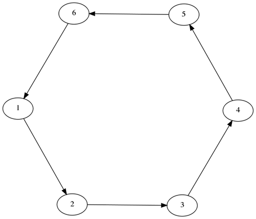
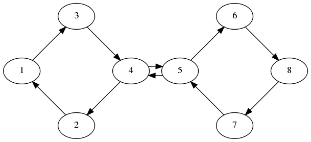
3 Gene Regulatory Networks were simulated from ODE models. The topologies are shown below:

Chain

Fully linear example
Figure 1: Chain

Ring

Contains non-linearities

Figure 2: Ring

Double Ring

Fully linear example

Figure 3:Double Ring

The State Space Representation

The general form of a state space model for gene expression is given by:
Equation 1:

[math]\displaystyle{ \dot{x} = Ax + Bu }[/math]

Equation 2:

[math]\displaystyle{ y = Hx }[/math]

• Where [math]\displaystyle{ \bar x_t = \begin{pmatrix} x_t \\ y_t \end{pmatrix} }[/math]
• [math]\displaystyle{ x_t }[/math] is a vector of hidden variables (length [math]\displaystyle{ T }[/math]) with hidden space dimensionality [math]\displaystyle{ k }[/math].
• [math]\displaystyle{ y_t }[/math] is a vector of observed quantities (length [math]\displaystyle{ T }[/math]) with dimensionality [math]\displaystyle{ p }[/math]. (i.e. This quantity will have a dimensionality equal to the number of observed genes).
• [math]\displaystyle{ u_t }[/math] is a D-dimensional vector of external driving inputs (length [math]\displaystyle{ T }[/math]).
• [math]\displaystyle{ A }[/math] is the matrix of dynamical interactions.
• [math]\displaystyle{ B }[/math] is a matrix of external driving inputs.
• [math]\displaystyle{ H }[/math] is a matrix of observations in the form [0 I] where I is [math]\displaystyle{ pxp }[/math] dimensional identity matrix, with dimensions dependent on the number of observed states [math]\displaystyle{ p }[/math]

The Ring Network

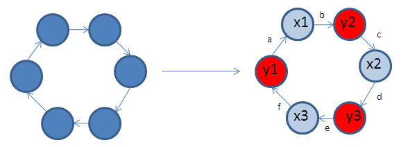
A biological example can be used to illustrate the representation above.Consider a real network containing 6 genes, regulating each other as shown in Figure 4.A. If we assume that in a real microarray experiment, we can only measure three out of 6 genes (Figure 4.B), this network then translates to the state space representation in Equation 3.

Figure 4:
A. This ring networks contains 6 genes, each represented by a node. B. The red nodes correspond to the measured genes [math]\displaystyle{ y }[/math], and the blue nodes correspond to the hidden genes [math]\displaystyle{ x }[/math]. Interactions between genes are represented by parameters [math]\displaystyle{ a,b,c,d,e,f }[/math].

Since in this particular example we have three hidden states and three measured states and three hidden states, the system can be represented as follows:
Equation 3:

[math]\displaystyle{ \begin{pmatrix}x1_{t+1} \\ x2_{t+1} \\ x3 _{t+1} \\ y1_{t+1} \\ y2_{t+1} \\ y3_{t+1} \end{pmatrix}= \begin{pmatrix} deg_{x1} & 0 & 0 & a & 0 & 0 \\ 0 & deg_{x2} & 0 & 0 & c & 0 \\ 0 & 0 & deg{x3} & 0 & 0 & e \\ b & 0 & 0 & deg_{y1} & 0 & 0 \\ 0 & d & 0 & 0 & deg_{y2} & 0 \\ 0 & 0 & f & 0 & 0 & deg_{y3} \end{pmatrix} \begin{pmatrix}x1_{t} \\ x2_{t} \\ x3 _{t} \\ y1_{t} \\ y2_{t} \\ y3_{t} \end{pmatrix} }[/math]

where the diagonal parameters [math]\displaystyle{ deg }[/math] represent the intrinsic degradation rates of every variable in the system.Since we only have three observed states, this is what our observation matrix would look like:
Equation 4:

[math]\displaystyle{ \begin{pmatrix} y1_{t} \\ y2_{t} \\ y3 _{t} \end{pmatrix} = \begin{pmatrix} 0 & 0 & 0 & 1 & 0 & 0 \\ 0 & 0 & 0 & 0 & 1 & 0 \\ 0 & 0 & 0 & 0 & 0 & 1\end{pmatrix} }[/math]