User:Nuri Purswani/Network/Methods
| Home | Introduction | Synthetic Datasets | Methods | Results | Discussion | References |
In this project, 2 types of network reconstruction methods were compared:
Bayesian Networks
Principle
Bayesian networks are widely used for modelling gene expression data, as they have a number of features that make them ideal candidates such as:
- Their ability to handle missing and noisy data
- Their ability to deal with hidden variables such as protein levels having an effect on observed mRNA expression levels, allowing them to make causal inferences on observed data from probability models (bioinf and medical infs and Friedman 25 med infs)
They can be described as follows:
If we consider 3 nodes representing each gene “A”, “B” and “C” as seen in Figure 1, their joint probability function is described in Equation 1.
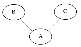
Figure 1: Static Bayesian Networks
In static Bayesian networks, the laws of conditional independence (ref) apply. This means that their joint probability distribution is given by:
Equation 1.
Every node is conditionally independent of its non-descendants, given its parents. This means that [math]\displaystyle{ A }[/math] and [math]\displaystyle{ B }[/math] are dependent on [math]\displaystyle{ C }[/math], but independent of their children. The drawback posed by the assumption of conditional independence in static Bayesian networks lies in their inability to cope with feedback loops. Therefore, dynamic Bayesian networks are better candidate models for gene expression. Dynamic Bayesian Networks (Murphy Mian 18 Bionfs and medical informatics) are more suitable for this purpose, as they can represent time series. Common examples of DBNs include Hidden Markov Models (reference) or Kalman Filter models- also referred to as linear Gaussian state space models (ref bioinfs and med infs 21, 22, 23, 5, 17). The Bayesian method of comparison we have chosen (Beal 2005) uses a Linear Gaussian State Space Model for gene expression, described in a very general form in the Inputs section.
Inputs and Outputs
Consider a state vector [math]\displaystyle{ \bar{x_t}= \begin{pmatrix} xt \\ yt \end{pmatrix} }[/math], where
Equation 2:
Equation 3
Further explanations of the variables and the model can be found in (Rangel et al. 2005. Chapter 9- Bioinformatics and Medical Informatics).
The matrix Ao contains the substructure below:
Equation 4:
[math]\displaystyle{ A_o = \begin{pmatrix} A & B \\ CA & CB+D \end{pmatrix} }[/math]
Where [math]\displaystyle{ A, B, CA, CB+D }[/math] are the variables from the state space model (See Rangel et al. 2005, Beal et al.).
The quantitiy of interest to us is the matrix CB + D, as it represents interactions between any given genes [math]\displaystyle{ i }[/math] and [math]\displaystyle{ j }[/math] in the network.
This method uses the z-statistic as a test for significant interactions. To look for the presence of an interaction, we perform the following tests:
- [math]\displaystyle{ H_o }[/math] = Any given entry in the CB+D matrix contains [math]\displaystyle{ μ=0 }[/math];
- [math]\displaystyle{ H_1 }[/math] = Reject null hypothesis.
If in any entry of CB + D we are able to reject [math]\displaystyle{ H_o }[/math] for any particular confidence interval of choice, we can consider it to be a significant interaction between two quantities. The CB+D matrix contains the "boolean structure" of the network. The main difference between this matrix and the dynamical structure function in the robust control method is that the CB+D matrix contains self-loops. In the dynamical structure function, we only consider interactions between adjacent genes and ignore self loops, so the dynamical structure function contains zeros in its diagonal.
Algorithm’s Requirements
This algorithm requires:
- Time series data
- A gaussian noise input perturbation.
In order for the algorithm to infer the correct structure, it must satisfy four properties:
- Stability. This property is characterized by convergence of trajectories to a fixed point. In order for the system to satisfy this criterion, the spectral radius of eigenvalues of the matrix must be < 1- since this is a discrete time system.
- Controllability: Complete state controllability (or simply controllability if no other context is given) describes the ability of an external input to move the internal state of a system from any initial state to any other final state in a finite time interval.
- Observability : This refers to a measure of how well the internal states of the system can be inferred, given the output observations. Formally, a system is said to be observable if, for any possible sequence of state and control vectors, the current state can be determined in finite time using only the outputs.
- Identifiability: If we apply a transformation to the state vector, as seen in (Rangel et al. 2005, Page 280), the system is identifiable if the observations generated by the coordinate transformation are identically distributed to the unmodified ones.
For additional theoretical explanations of these terms see Ljung 1987.
Assumptions
These types of methods use linear dynamical systems (Rangel et al. 2005) to model time series data. These are a type of dynamic bayesian networks extensively used in areas of control and signal processing. Here, they assume that the models for gene expression:
- Are linear time invariant
- Contain gaussian noise
- Hidden variables evolve with Markovian dynamics.
We previously described a state space representation for this type of model :synthetic datasets. Here, we add a variation to its definition by defining a discrete-time state space model, where external driving inputs are replaced by Gaussian noise. This is what perturbs the system.
Choice of method of comparison
The authors of this method for network inference using hidden variables published two methods of Bayesian inference:
- Rangel et al. Uses linear gaussian state space models and a bayesian inference approach to estimate the maximum likelihood of parameters, improving accuracy by using many bootstrapping samples and increasing the number of repeats.
- Beal et al. Uses linear gaussian state space models and a variational bayesian inference approach where instead of estimating point parameters, it applies the [jensen inequality http://en.wikipedia.org/wiki/Jensen%27s_inequality] to the lower bound of the marginal likelihood of each parameter in the model. This way, it is able to estimate a posterior distribution from the initial guess of the prior.
Both methods use the (http://en.wikipedia.org/wiki/Expectation-maximization_algorithm expectation-maximization) algorithm to optimize their guesses.
In the initial implementations , of the project, our candidate network structures were fed to both methods to compare and contrast network structure. However, after some implementations and recommendation from the authors, Beal’s was the method of choice over Rangel’s for this comparison. The reason for the choice was that:
- The general likelihood method is prone to overfitting. This is specially the case where models have too many variables and relatively small numbers of samples.
- In order to avoid overfitting of data, Beal’s method assumes the existence of a prior distribution p(theta) where theta is every parameter in the model and aims to estimate hyperparameters of the distribution as opposed to providing a point estimate of A.
- As illustration, assume that parameter A is beta distributed- Rangel’s method will try to estimate A directly, while Beal’s method will estimate hyperparameters of distribution of A.
Note that both methods suffer from the tendency of overfitting when there are too many variables and not enough samples (Beal 2007). In addition, as outlined by the authors they will perform badly when:
- Dynamics and output processes are time invariant, which is unlikely in a real biological system.
- The time slices are not spaced linearly, so there may be non linearities in the rate of the transcriptional processes that we miss out.
- The noise of the dynamics and the output may not be Gaussian, whereas this algorithm assumes it is the case.
Rangel's method is rigid to non-linearities which is another reason why it was not chosen for the comparison.
Diagram
This summarises the main steps of Beal’s inference algorithm. More detail can be found in the references, so this diagram is only a visual explanation of how the algorithm works. See Beal 2005 for a better explanation of the symbols and parameters:
- y- observed variables, x- latent variables and theta-parametesr.
- Marginal likelihood of a given model-
- P(y|M)=ingeralp(y,x,theta|m)dthetadx tells how well a particular model fits data, as opposed to the maximum likelihood, which forms the basis. Computationally intractable though, so use jensen’s inequality to maximize the lower bound of the likelihood.
- Find lower bound of marginal likelihood that maximizes the KL divergence between the approximation qthetaqx and the true posterior pxtheta given that.
- VBE step- estimates hidden state dimension
- VBM step/ Bayesian distribution of parameters- Occam’s razor.
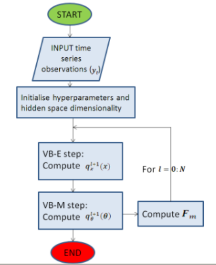
Figure 2:Very simplified summary of Beal's algorithm. The details have been ommitted, but are explained extensively in his PhD thesis.
Robust Control Method (Gonçalves et al. 2008) reference conference papers
Principle
Algorithmic methods for biological network inference attempt to recover network structure directly from observations, by repeating experiments multiple times. This method, based on the principles of robust control relies on external inputs that perturb the individually observed quantities of the system at every time-step. Furthermore, while network inference algorithms like Beal's make inferences about hidden states in the system and aim to recover the full state space representation, Gonçalves and Warnick (2008) introduce the notion of a "dynamical structure function", which describes relationships between observed nodes, describing any connection between them as indirect, as shown in Figure 3:
A B.
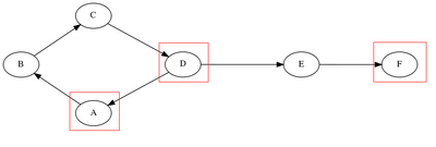
![]() Figure 3 left, full network, measured quantities circled in red. The algorithm recovers the relationship between observed quantities, which can be interpreted as an "indirect" reaction.
Figure 3 left, full network, measured quantities circled in red. The algorithm recovers the relationship between observed quantities, which can be interpreted as an "indirect" reaction.
Gonçalves and Warnick also outlined the necessary and sufficient conditions to recover biological network structure between the observed nodes. They provided mathematical proofs that showed that even if the system's transfer function can be recovered from input output data it is not possible to infer the dynamical network structure without any extra information.
As illustrated by Example 1, from the paper:
A system with a transfer function given by
is consistent with systems [math]\displaystyle{ A_1 }[/math] and [math]\displaystyle{ A_2 }[/math], with very different internal dynamical structures. These are known as minimal realisations.
To overcome this problem, they propose in (MIT book) a way of designing biological experiments, that requires perturbing each species in turn. As shown below:
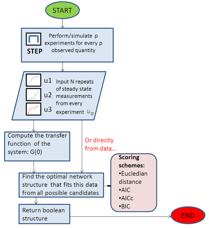
1. If a network contains p measured species, the same number p of experiments must be performed.
2. Each experiment must independently control a measured species (see figure 4)
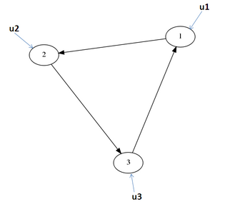
Figure 4: Input a perturbation at each measured state When previous information is known about the network, these conditions can be relaxed. See (paper) for a rigorous proof. Experiments such as gene silencing with RNA interference or inducible overexpression can be used to control each observed species in turn with a known input.
Inputs and Outputs
In synthetic datasets we introduced the state space representation in continuous-time form as:
Equation 5:
Equation 6:
The state space representation can be further partitioned into a function of the hidden and measured states, as shown in Equation 7:
Equation 7
By taking Laplace transforms of the signals above, and after some mathematical simplification (see full derivation in Gonçalves et al.), we can obtain a dynamical structure function which describes the relationship between the external inputs to the system and the observed states:
Equation 8:
where [math]\displaystyle{ Q }[/math] is the internal structure matrix of the system, and [math]\displaystyle{ P }[/math] is the control structure matrix.
Equation 9:
Notice that the internal structure [math]\displaystyle{ Q }[/math] contains zeros in its diagonal. This method ignores self-loops in individual quantities, but instead focuses on obtaining a matrix of direct/indirect interactions between observed species. P is a matrix of driving inputs (steps) and only contains entries in the diagonal.
This algorithm can take two types of data: steady state and time series. Provided that experiments have been performed as described earlier, with a steady state input it is able to recover the boolean structure of the observed quantities in the network. With a time series, it is capable of recovering the dynamical structure function, containing more detail about the relationships between interacting species. The "Boolean" structure simply refers to [math]\displaystyle{ Q(0) }[/math], and simply tells us if there is a direct/indirect reaction between the two quantities. In this project, the time series code was not yet available, so this algorithm was implemented using steady state measurements from an insilico model.
In Summary
- This algorithm can take the following inputs:
- Steady state
- Time series
- It requires that a number [math]\displaystyle{ p }[/math] of experiments are performed on every [math]\displaystyle{ p }[/math] measured species, else it is unable to recover the network.
- This algorithm will output:
- The Boolean network structure between observed quantities if provided with steady state data.
- The Full Dynamical structure function (i.e the transfer function between every single interacting species) if provided with time series data.
Note: In this project we have implemented the steady state version of the algorithm, so this is what will be used for the comparison
Assumptions
- The network is assumed to be Linear Time Invariant. In reality, biological networks are non linear, and their dynamics are constantly changing.
- Although it makes no a priori assumptions (sparsity/parsimony) about the input data, the preferred scoring scheme (AICc) tends to penalize too many connections, favouring the simpler network designs. In biology, there is evidence that gene regulatory networks are not necessarily optimal. Through the course of evolution, biological pathways have emerged as a result of indirect reactions. Therefore, this method still lacks biological relevance.
- It ignores the presence of self loops (auto-catalysis, degradation) and only considers biological interactions between neighbouring quantities. This limits its usefulness in biological mechanisms that heavily rely on self enhancement (e.g. pattern formation)
Diagram
Scoring Method:Choosing the best network
The following distance measures and information criteria were used to rank networks accordingly: Eucledian Distance, Akaike's Information Criteria( AIC and AICc- a variation of it) and the Bayesian Information Criterion (BIC)

