Lucia I. Ramirez Week 12
From OpenWetWare
Jump to navigationJump to search
Using YEASTRACT to Infer which Transcription Factors Regulate a Cluster of Genes
- Opened the gene list (file name: wt_profile37_genelist) in Excel for the profile/cluster that I analyzed for the Week 11 Assignment.
- Copied the list of gene IDs onto my clipboard.
- Launched a web browser and go to the YEASTRACT database.
- On the left panel of the window, clicked on the link to Rank by TF.
- Pasted my list of genes from my cluster into the box labeled ORFs/Genes.
- Checked the box for Check for all TFs.
- Accepted the defaults for the Regulations Filter (Documented, DNA binding plus expression evidence)
- Did not apply a filter for "Filter Documented Regulations by environmental condition".
- Ranked genes by TF using: The % of genes in the list and in YEASTRACT regulated by each TF.
- Clicked the Search button.
- Questions:
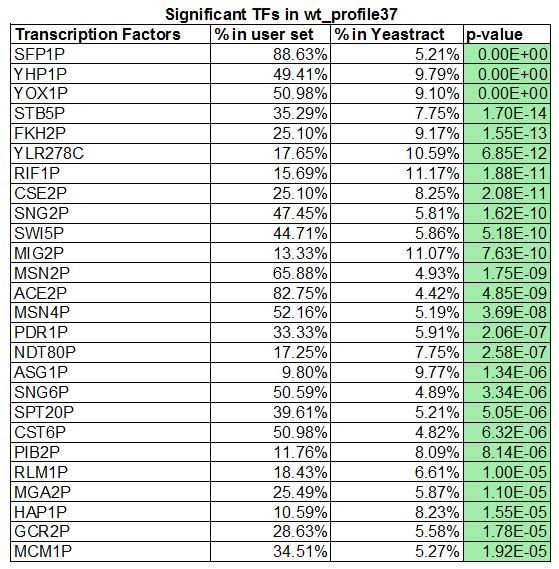
- In the results window that appears, the p values colored green are considered "significant", the ones colored yellow are considered "borderline significant" and the ones colored pink are considered "not significant". How many transcription factors are green or "significant"?
- There are 26 significant transcription factors
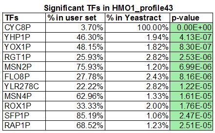
- List the "significant" transcription factors, along with the corresponding "% in user set", "% in YEASTRACT", and "p value".
- How many of the transcription factors appear in both of your lists?
- SFP1P, YHP1P, YOX1P, YLR278C, MSNP2, and MSN4P, a total of 6 common transcription factors. 26 transcription factors were generated in my wt_list and 11 were generated in Lauren's HMO1_list. We decided to focus on the mutant gene, in which we added CIN5, GLN3, HMO1 and ZAP1 to have a total of 15 transcription factors.
- Went back to the YEASTRACT database and followed the link to Generate Regulation Matrix.
- Copy and pasted the list of transcription factors I identified (plus CIN5, GLN3, HMO1, and ZAP1) into both the "Transcription factors" field and the "Target ORF/Genes" field.
- Generated several regulation matrices, with different "Regulations Filter" options.
- First one: accepted the defaults: "Documented", "DNA binding plus expression evidence"
- Clicked the "Generate" button.
- In the results window that appears, I clicked on the link to the "Regulation matrix (Semicolon Separated Values (CSV) file)" that appears and saved it to my Desktop. Renamed this file with a meaningful name.
- Repeated these steps to generate a second regulation matrix, this time applying the Regulations Filter "Documented", "Only DNA binding evidence".
- Repeated these steps a third time to generate a third regulation matrix, this time applying the Regulations Filter "Documented", DNA binding and expression evidence".
- In the results window that appears, the p values colored green are considered "significant", the ones colored yellow are considered "borderline significant" and the ones colored pink are considered "not significant". How many transcription factors are green or "significant"?
Analyzing and Visualizing Your Gene Regulatory Networks
I analyzed the regulatory matrix files generated above in Microsoft Excel to visualize them using GRNsight to determine which one will be appropriate to pursue further in the modeling.
- First formated the output files from YEASTRACT. Repeated these steps for each of the three files generated above.
- Opened file in Excel.
- It will not open properly in Excel because a semicolon was used as the column delimiter instead of a comma. To fix this, Select the entire Column A. Then go to the "Data" tab and select "Text to columns". In the Wizard that appears, select "Delimited" and click "Next". In the next window, select "Semicolon", and click "Next". In the next window, leave the data format at "General", and click "Finish". This should now look like a table with the names of the transcription factors across the top and down the first column and all of the zeros and ones distributed throughout the rows and columns. This is called an "adjacency matrix."
- Saved this file in Microsoft Excel workbook format (.xlsx).
- Checked to see that all of the transcription factors in the matrix are connected to at least one of the other transcription factors by making sure that there is at least one "1" in a row or column for that transcription factor.
- If a factor is not connected to any other factor, delete its row and column from the matrix. Make sure that you still have somewhere between 15 and 30 transcription factors in your network after this pruning.
- For this adjacency matrix to be usable in GRNmap (the modeling software) and GRNsight (the visualization software), we need to transpose the matrix. Inserted a new worksheet into your Excel file and named it "network". Went back to the previous sheet and selected the entire matrix and copy it. Went to my new worksheet and clicked on the A1 cell in the upper left. Selected "Paste special" from the "Home" tab. In the window that appears, check the box for "Transpose".
- The labels for the genes in the columns and rows match. (Deleted the "p" from each of the gene names in the columns.) Adjusted the case of the labels to make them all upper case.
- Inserted text "rows genes affected/cols genes controlling" into cell A1.
- Opened file in Excel.
- Repeated these steps for each of the three gene regulatory matrices generated above.
- Created a new worksheet and called it "degree". Copy and pasted adjacency matrix from the "network" sheet into this new worksheet.
- Found number of genes that the transcription factor in that column is controlling, or the out-degree.
- In the first empty cell at the bottom of column A, typed "Out-degree". In the cell to the right of that (in Column B), I typed the equation
=SUM(and selected the range of cells in column B that has 1's and 0's in it, closed the parentheses, and pressed Enter. Copy and pasted that equation across all of the columns.
- In the first empty cell at the bottom of column A, typed "Out-degree". In the cell to the right of that (in Column B), I typed the equation
- Found number of transcription factors that regulate the gene in that row, or the in-degree.
- In the first empty column in Row 1 to the right of the adjacency matrix, type "In-degree". In Row 2 of this column, type the equation
=SUM(and select the entire row of 1's and 0's, close the parentheses, and press Enter. Copy and paste the equation down the entire column, including the row that contains the out-degree sums.
- In the first empty column in Row 1 to the right of the adjacency matrix, type "In-degree". In Row 2 of this column, type the equation
- The number in the lower right-hand corner, the sum of sums, is the total number of edges in the adjacency matrix.
- There was a total of 74 number of edges for the DNA binding plus expression evidence data set.
- There was a total of 31 edges for the Only DNA binding evidence data set.
- There was a total of 7 edges for the DNA binding and expression evidence data set.
- Plotted the degree distributions for each of my gene regulatory networks. In the "degree" worksheet, I created three columns to the right titled "Frequency", "In-degree total", and "Out-degree total". In the "Frequency" column, I numbered sequentially from 1 to the largest degree number in my calculations above (The 12th degree was the largest for the DNA binding plus expression evidence data set). In the "In-degree total" column, type the number of genes with that in-degree for each of the frequencies. In the "Out-degree total" column, I typed the number of genes with that out-degree for each of the frequencies.
- Selected the "In-degree total" and "Out-degree total" columns. Went to the "Insert" tab and selected the vertical bar chart type to insert a plot of the degree distribution. See figures in powerpoint presentation below.
- Visualized these gene regulatory networks with the GRNsight software.
- Went to the GRNsight home page.
- Selected the menu item File > Open and select one of the regulation matrix .xlsx file that has the "network" worksheet in it as formatted above. Repeated with the other two regulation matrix files.
- Results
- Significant transcription factors in each gene profile were determined by the p-value. Choosing to focus on the mutant gene's profile #43 with 11 significant transcription factors, we created three candidate gene regulatory networks by using the GRNsight software by changing the regulation filters from "DNA binding plus expression evidence" to "Only DNA binding evidence" then to "DNA binding and expression evidence". All three networks were viewed in excel spreadsheets where the total number of edges and degree distribution was determined. A "1" in a cell meant there was a connection between the transcription factor in that row with that column. The data set with regulation filter "DNA binding and expression evidence" had three transcription factors that showed no connection, which were then deleted. "DNA binding plus expression evidence" had the most number of edges. There was also a large concentration of activity in the third degree for both "DNA binding plus expression evidence" and "Only DNA binding evidence" data sets. I would choose the "DNA binding plus expression evidence" for the modeling since there are more edges, which gives us the ability to see possible trends. See PowerPoint slides below for visuals.
HMO1 Network: DNA binding PLUS expression evidence
HMO1 Network: ONLY DNA binding evidence
HMO1 Network: DNA binding AND expression evidence
Back to User page: Lucia I. Ramirez
Journals/Assignments
Week 1
Week 2
Week 3
Week 4
Week 5
Week 6
- Assignment
- Week 6 Individual Journal Not Assigned
- Class Journal Entry
Week 7
Week 8
Week 9
Week 10
Week 11
Week 12
Week 13
Week 14
Week 15

