HRV:Signal Processing

Home        Lab Members        Physiological Systems        Monitoring Parameters in the ICU        ECG        HRV        Clinician's Perspective        Cardiorespiratory Monitors        Signal Processing        Deliverables        Journal        Abbreviations       

Signal Processing

In order to create an algorithm that is able to accurately extract HRV and use it in a way which is useful to a clinician, the signal processing is broken down into the following steps:

1. Obtaining ECG data from archives
2. Using this data to plot a typical ECG waveform
3. Removal of noise
4. Detection of the R wave peak
5. Extrapolation of R wave peak to HRV in the time domain
6. Linking this is changes in physiological signal to predict medical events

More steps may be added through the process depending on what is found at each stage.

The team will be using Python to accomplish this.

Coding Plan

Our Coding Plan

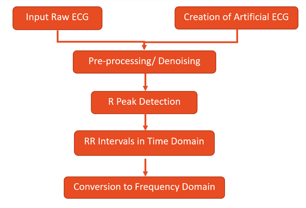
Evolution of our Code

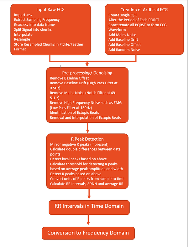
A more detailed guide to the steps included in the code can be seen in the diagram below.

A More Detailed View of Our Coding Plan

Opening a .csv File

Figure 2.1a: Step 1a of signal processing pipeline, the input ECG module.

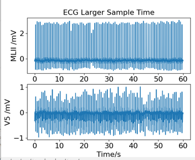
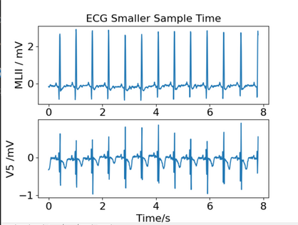
Opening a .csv file and printing the ECG data, https://github.com/cay15/hrv/blob/master/52.py The ECG dataset which was used to produce these plots is the MIT-BIH Normal Sinus Rhythm Sample No.16265.

• 

  Input and Display Larger Sample of ECG

• 

  Input and Display Smaller Sample of ECG

Figure 2.1b: ECG plots on larger (left) and shorter (right) sample times

Pre-Processing

Figure 2.2a: Pre-processing steps in the input ECG module.

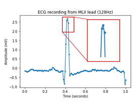
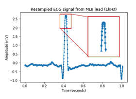
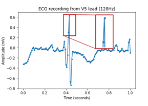
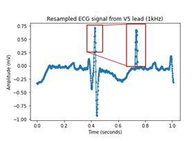
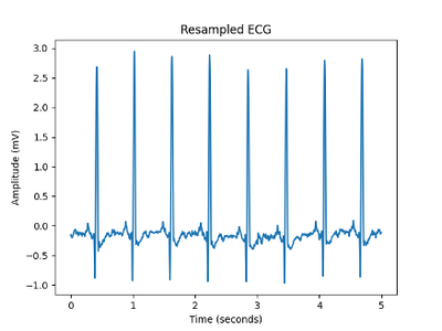
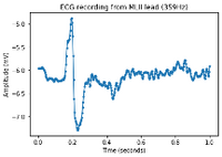
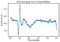
We obtain the original sampling frequency of the data from the .csv file and resample the waveform to 1000Hz, so that it is consistent over different inputs, (see https://github.com/cay15/hrv/blob/master/upsample_ecg.py). This also splits the signal so a smaller, more manageable chunk is passed to the other modules. The ECG dataset which was used to produce these plots is the MIT-BIH Normal Sinus Rhythm Sample No.16265 .

• 
• 

• 
• 

Figure 2.2b: The first QRS wave of the ECG before and after resampling.

Artificial ECG

Figure 2.3a: Pre-processing steps in the input ECG module.

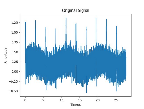
Creating an artificial ECG to test out the filtering and peak detection modules, https://github.com/cay15/hrv/blob/master/fakeecg.py. The ECG QRS segment is modelled by a Daubechies wavelet, while the rest of the wave is given by an interval of rest. Gaussian noise and sinusoids of various frequencies are added to simulate mains noise, electromyogram noise, and baseline offset.

Figure 2.3b: Section of the Artificial ECG corrupted by noise

Filtering

Figure 2.4a: Steps in the filter ECG module.

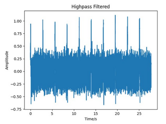
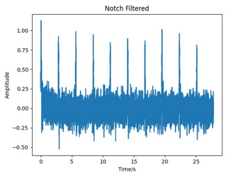
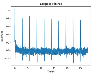
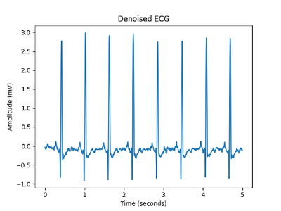
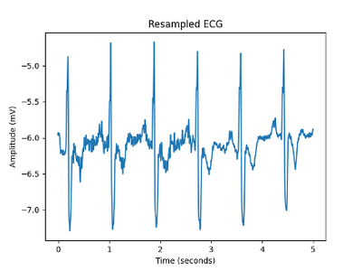
Testing out filtering methods including a notch filter, high pass and low pass, https://github.com/cay15/hrv/blob/master/filter.py . The notch filter is designed to remove mains interference at 50Hz. The low pass filter is designed to remove electromyogram noise and other high-frequency noise with a cutoff of 150Hz. The high pass filter is designed to remove baseline drift and other low-frequency noise with a cutoff of 0.5Hz.

• 

  Figure 2.4b: Artificial ECG with High Pass Filter Applied with a cutoff frequency of 0.5Hz

• 

  Figure 2.4c: Notch Filter applied to the previous signal to remove 50Hz signal

• 

  Figure 2.4d: Low Pass Filter applied to the previous signal to remove signals above 150Hz

R Peak Detection

Figure 2.5a: Steps in the R Peak Detection module.

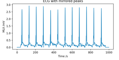
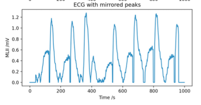
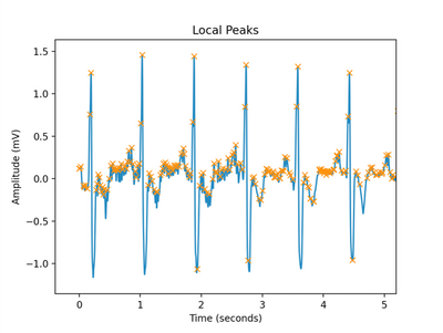
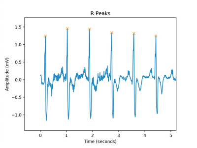
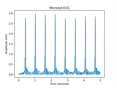
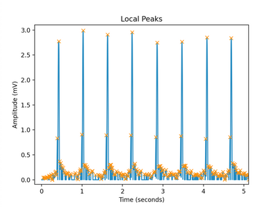
1. Peak detection module which finds peaks based on whether surrounding samples have greater amplitudes than it, mirrors these peaks, for the case where peaks are inverted from medical conditions or lead placement. It then uses boundaries which can be specified to rule out peaks that are too close together by specifying a minimum amplitude, https://github.com/cay15/hrv/blob/master/peak_detection.py.

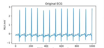
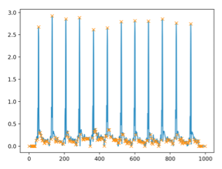
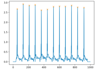
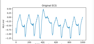
Here are the results obtained using a normal sinus rhythm ECG, the peaks are very clearly and accurately detected. The data used was from the MIT-BIH Normal Sinus Rhythm Database .

• 

  Figure 2.5b: Original ECG of Patient with Normal Sinus Rhythm

• 

  Figure 2.5c: Previous ECG with Mirrored Peaks

• 

  Figure 2.5d: All Points where the Amplitude Increases by a Specified Amount Denoted by Orange Points

• 

  Figure 2.5e: Peaks Detected after the Application of Boundaries for Each Peak

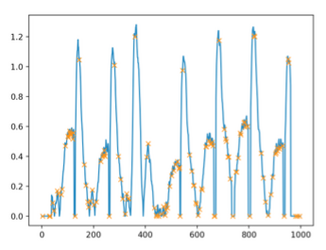
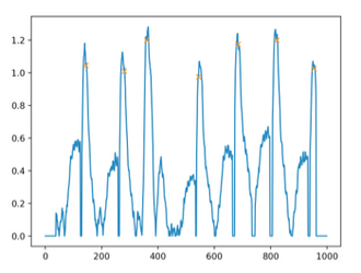
The sample used below is from the MIT-BIH Malignant Ventricular Database and was used to test the module on a much more difficult ECG than normal sinus rhythm.

• 

  Figure 2.5f: Original ECG of Patient with Malignant Ventricular Ectopy

• 

  Figure 2.5g: Previous ECG with Mirrored Peaks

• 

  Figure 2.5h: All Points where the Amplitude Increases by a Specified Amount Denoted by Orange Points

• 

  Figure 2.5i: Peaks Detected after the Application of Boundaries for Each Peak

The application of boundary conditions is not perfect and needs tweaks in order to be as accurate as possible.

Modules Combined

These functions have been combined to one main python script which takes in the .csv file, resamples it, removes noise and detects the peaks, https://github.com/cay15/hrv/blob/master/main.py

The previous code has been amended to allow more user input in terms of deciding whether to sample an artificial ECG or a raw .csv file and if it is a raw file, which lead of the ECG to process, https://github.com/cay15/hrv/blob/master/main12.py.

Waveform Results

Normal Sinus Rhythm

Figure 3.1: A 60 second ECG recording of a person with normal sinus rhythm as measured by one ECG lead from the MIT-BIH ECG database.

Figure 3.2: First 5s of the resampled ECG, with slight baseline drift

Figure 3.3: First 5s of denoised ECG, with baseline drift removed

Figure 3.4: First 5s of mirrored ECG

Figure 3.5: First 5s of ECG with local peaks detected

Figure 3.6: R peaks distinguished among local peaks

Figure 3.7: Scatter plot of RR intervals against elapsed time of ECG recording

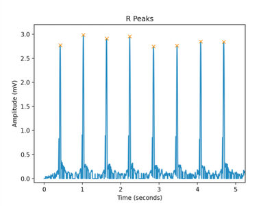
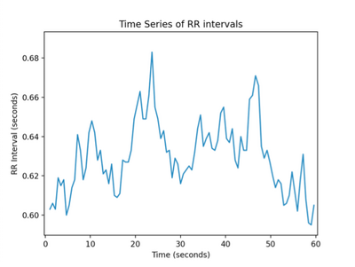
Arrythmia

Figure 4.1: A 60 second ECG recording of a person with normal sinus rhythm as measured by one ECG lead from the MIT-BIH ECG database.

Figure 4.2: First 5s of the resampled ECG, with slight baseline drift

Figure 4.3: First 5s of denoised ECG, with baseline drift removed

Figure 4.4: First 5s of mirrored ECG

Figure 4.5: First 5s of ECG with local peaks detected

Figure 4.6: R peaks distinguished among local peaks

Figure 4.7: Scatter plot of RR intervals against elapsed time of ECG recording

Atrial Fibrillation

Figure 5.1: A 60 second ECG recording of a person with normal sinus rhythm as measured by one ECG lead from the MIT-BIH ECG database.

Figure 5.2: First 5s of the resampled ECG, with slight baseline drift

Figure 5.3: First 5s of denoised ECG, with baseline drift removed

Figure 5.4: First 5s of mirrored ECG

Figure 5.5: First 5s of ECG with local peaks detected

Figure 5.6: R peaks distinguished among local peaks

Figure 5.7: Scatter plot of RR intervals against elapsed time of ECG recording

Malignant Ventricular Ectopy

Figure 6.1: A 60 second ECG recording of a person with normal sinus rhythm as measured by one ECG lead from the MIT-BIH ECG database.

Figure 6.2: First 5s of the resampled ECG, with slight baseline drift

Figure 6.3: First 5s of denoised ECG, with baseline drift removed

Figure 6.4: First 5s of mirrored ECG

Figure 6.5: First 5s of ECG with local peaks detected

Figure 6.6: R peaks distinguished among local peaks

Figure 6.7: Scatter plot of RR intervals against elapsed time of ECG recording

Noise Stress Test

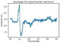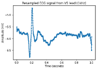Figure 7.1a: The first QRS wave at original sampling frequency of 359Hz	Figure 7.1b: The first QRS wave in Fig 7.1a after resampling at 1000Hz

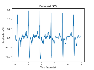Figure 7.2a: Resampled ECG before denoising, baseline drift present	Figure 7.2b: ECG after denoising

Figure 7.3a: Local peaks detected on ECG	Figure 7.3b: R peak detection from local peaks

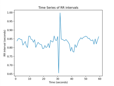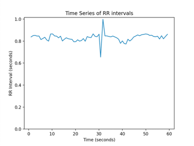
Figure 7.4a: Scatter plot of RR interval distribution with y-axis interval [0,1.0]	Figure 7.4b: Scatter plot of RR interval distribution with y-axis interval [0.65,1.00]

References

- ↑ 1.0 1.1 1.2 1.3 Goldberger AL, Amaral LAN, Glass L, Hausdorff JM, Ivanov PCh, Mark RG, Mietus JE, Moody GB, Peng C-K, Stanley HE. PhysioBank, PhysioToolkit, and PhysioNet: Components of a New Research Resource for Complex Physiologic Signals. Circulation 101(23):e215-e220 [Circulation Electronic Pages; http://circ.ahajournals.org/content/101/23/e215.full]; 2000 (June 13).
- ↑ 2.0 2.1 2.2 T. A. L. The Beth Israel Deaconess Medical Center, ‘The MIT-BIH Normal Sinus Rhythm Database’. physionet.org, 1990, doi: 10.13026/C2NK5R.
- ↑ S. D. Greenwald, ‘The MIT-BIH Malignant Ventricular Arrhythmia Database’. physionet.org, 1992, doi: 10.13026/C22P44.