Physics307L:People/Archer
Notebook
Report
none yet
Summary
Oscilloscope Lab
SJK 03:27, 17 September 2008 (EDT)

Overall, very good lab! Except for a couple things missing (noted on the raw data page), your notes are very details and your summary table is great.
The raw data from the lab is here.
In summary, I measured the peak-to-peak voltage and period of multiple sine waves of three different amplitudes the peak-to-peak voltage and period of a sine wave with a large DC offset, as well as the fall time of a DC Voltage read through AC coupling, measured by placing cursors at the peak of the function and at the 90% decay point of the function, as well as automatic calculation in the oscilloscope. I measured everything else by visual inspection, cursor inspection, and automatic calculation in the oscilloscope.
SJK 03:12, 17 September 2008 (EDT)

This table is a nice and succinct way to report your results...glad you decided to use it! It would probably be more readable if you combined the error with the measurements (e.g. "value ± error")...we'll talk about this during lecture soon.
I also think there are some typos in your error values for some entries (e.g. 5 +/- 5)
| MEASUREMENTS | Visual | Cursors | Calculate | ERROR | Visual | Cursors | Calculate |
|---|---|---|---|---|---|---|---|
| Pk-Pk 200 Hz | 500 mV | 508 mV | 504~508 mV | 100 mV | 16 mV | 1 mV | |
| Period 200 Hz | 5 ms | 5.2 ms | 5.128~5.144 ms | 5 ms | 0.8 ms | 0.001 ms | |
| Pk-Pk Hi-Amp | 2200 mV | 2220 mV | 2180~2200 mV | 200 mV | 80 mV | 10 mV | |
| Period Hi-Amp | 5 ms | 5.2 ms | 5.110~5150 mV | 5 ms | 0.8 ms | 0.001 ms | |
| Pk-Pk Lo-Amp | 60 mV | 59.2 mV | 60.0~63.2 mV | 20 mV | 3.2 mV | 0.1 mV | |
| Period Lo-Amp | 5 ms | 5.2 ms | 5.110~5.170 ms | 5 ms | 0.8 ms | 0.001 ms | |
| Pk-Pk Offset | 900 mV | 880 mV | 864~872 mV | 100 mV | 32 mV | 1 mV | |
| Period Offset | 5 ms | 5.2 ms | 5.130~5.140 ms | 5 ms | 0.8 ms | 0.001 ms | |
| Fall Time | n/a | 58 ms | 49.40~56.00 ms | n/a | 4 ms | 0.01 ms | |
| Time Constant | n/a | 26.3 ms | 24.0 ms | n/a | 1.8 ms | 1.5 ms |
I am satisfied with this result, since nothing seems to be too unexpected. I would attribute the fluctuations to random error. If I had more time, I might examine Fourier transform phenomena in the wave functions.
I am still confused by the nature of capacitive coupling. SJK 03:10, 17 September 2008 (EDT)

we can talk about this some more when you'd like
I did not explore anything outside of the lab parameters. I have no suggestions for this lab. SJK 03:26, 17 September 2008 (EDT)

This was a pretty straightforward lab, so it's fine not to have comments. However, this kind of thinking ("what would I do if I had more time to take better data?") is good thinking to practice, and you'll want to put some more effort into this in the future labs.
Planck's Constant Lab
SJK 12:38, 20 October 2008 (EDT)

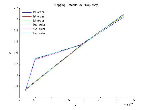
Good job on this lab. You took some very good stopping potential versus frequency data, and obtained a good final result with uncertainty. There are a couple problems. First, you had the wrong conclusion about the charging time, as far as the theory goes. Second, you are missing a description of your linear fitting methods. How did you treat those anomalous second order points? Did you use Matlab? This problem would have been solved if you had an additional page in your primary data notebook in which you took notes as you were analyzing the data.
The raw data for the lab can be found on the following pages:9/15/08 and 9/29/08.
In summary, I measured the stopping potentials (taken to be the maximum potentials measured) in a photodiode of multiple wavelengths of light diffracted from a mercury lamp at multiple levels of intensity, as well as the time taken to achieve this stopping potential for some of these wavelengths.
For Photon Theory Part A,
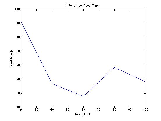
| Green Wavelength | 100% Intensity | 80% Intensity | 60% Intensity | 40% Intensity | 20% Intensity |
|---|---|---|---|---|---|
| Stopping Potential | 0.886~0.887 V | 0.886~0.887 V | 0.875 V | 0.873 V | 0.871 V |
| Mean Time to Reset | 48.20 s | 58.64 s | 38.00 s | 46.89 s | 91.08 s |
| Standard Deviation | 5.94 s | 3.82 s | 1.90 s | 0.34 s | 8.50 s |
| Number of Measurements | 5 | 5 | 3 | 3 | 3 |
For Photon Theory Part B,
| First Order | Yellow | Green | Blue | Violet | Ultraviolet |
|---|---|---|---|---|---|
| Mean Stopping Potential | 0.746 V | 0.885 V | 1.526 V | 1.752 V | 2.057 V |
| Standard Deviation | 0.005 V | 0.007 V | 0.009 V | 0.016 V | 0.016 V |
| Number of Measurements | 3 | 3 | 3 | 3 | 3 |
Passing different intensities of same-colored light has very little effect on stopping potential and thus very little effect on photon energy; the charging time therefore should not be affected.SJK 12:04, 20 October 2008 (EDT)

The second part is incorrect. In order for the capacitor to charge, electrons need to move from cathode to anode, and a fixed number of electrons are needed to get to a set voltage. One photon is required to move one electron. Thus, for lower photon rates (intensities), you expect lower charging rate (and longer charging time)
Longer wavelengths of light have lower stopping potentials, while higher shorter wavelengths have higher potentials, by extension, shorter wavelengths have higher energies.
This lab supports a photon-based model of light, since the wavelength (rather than the intensity) has the greatest effect on stopping potential by far.
The slight drop in stopping potential is possibly due to the physical limitations of the photodiode used to capture wavelengths, which may not function properly for low intensities of light.SJK 12:07, 20 October 2008 (EDT)

Exactly. In order to read the voltage, you must draw a small current from the device ... this "discharging" current is fixed and competed with the charging current. The lower the charging current (the lower the photon intensity), the more the discharging current matters.
For Determination of Planck's Constant,
| Second Order | Yellow | Green | Blue | Violet | Ultraviolet |
|---|---|---|---|---|---|
| Mean Stopping Potential | 0.731 V | 1.296 V | 1.544 V | 1.755 V | 2.091 V |
| Standard Deviation | 0.003 V | 0.013 V | 0.004 V | 0.001 V | 0.004 V |
| Number of Measurements | 3 | 3 | 3 | 3 | 3 |
SJK 12:10, 20 October 2008 (EDT)

These graphs are nice, but a few changes can make them much better. (1) individual data points instead of lines -- it's very tough to see the data points if they happen to be co-linear (2) better axes labels (title + units, for example ("frequency (Hz)") (3) Figure captions--captions help the reader understand the figure without having to find where in the text the figure is described.
The slope of this linear fit is h/e (Planck's constant over elementary charge) and the y-intercept is W0/e (Work function over elementary charge).
SJK 12:30, 20 October 2008 (EDT)

Looks like you got some very nice data! First a minor comment: You have too many digits on your numbers, which make them difficult to read. Since your error is 1 order magnitude less than your value, you can report it as, 6.6 +/- 0.5 J*s. Second, more importantly: you should compare to the accepted value by comparing the deviation from accepted value relative to your uncertainty. In the case of your values, it seems like your answer is quite consistent!
From these 6 data sets of V vs. ν, we obtain these values:
| Values | h | W0 | σ (h) | σ (W0) |
|---|---|---|---|---|
| Divided by e | 4.102e-15 J*s/C | 1.283 J/C | 3.2983-16 J*s/C | 0.267 J/C |
| Raw Value | 6.571e-34 J*s | 0.205e-18 J | 5.284e-35 J*s | 4.285e-20 J |
Compared with the accepted value of 6.626e-34 J*s for h, this value obtained in the experiment is quite close, and is on exactly the right order of magnitude.
These results seem good, aside from the low-intensity anomalies in the first part of the experiment, through which error crept in. If I had more time, I might examine the intensity relationship for other wavelengths. I did take extra measurements in addition to what the experiment demanded, to get more accurate results.
Poisson Distribution Lab
SJK 02:18, 1 November 2008 (EDT)

You did a very good job acquiring data for this lab (but your raw data isn't shown anywhere!). You also did a good job analyzing the data initially (but your analysis code is not shown. I can see that you did a lot of work, but actually between this summary and your primary lab notebook, the description of that work is missing, thus making it tough to assess your methods. As one example: this is the Poisson distribution lab and you don't anywhere talk about the formula for the Poisson distribution. Nor do you explicitly say anything about the distribution (though you do allude to the mean = variance property via your analysis)...do you see what I mean?
The relevant pages of the lab notebook are 10/1/08, 10/3/08, and 10/6/08.
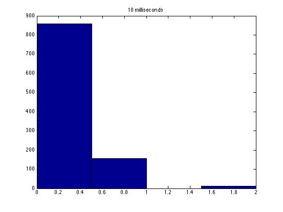
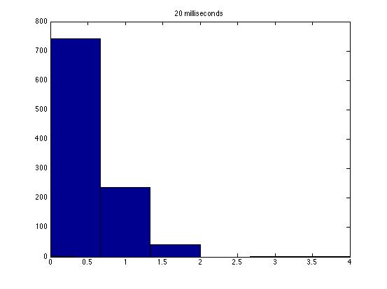
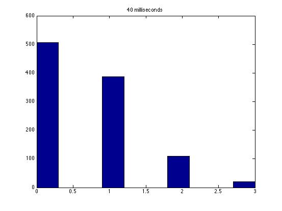
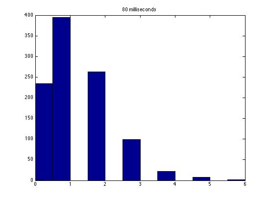
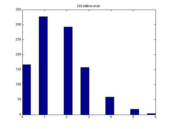
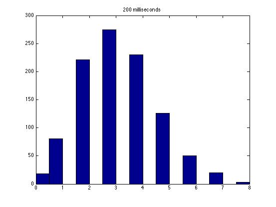
In this lab, I measured counts of background radiation with a photomultiplier tube. I took multiple readings with multiple dwell times.
SJK 02:08, 1 November 2008 (EDT)

You apparently are using matlab for analysis...make sure to upload your code in your primarly lab notebook and to have notes in your primary notebook about how you analyzed the data!
SJK 02:15, 1 November 2008 (EDT)

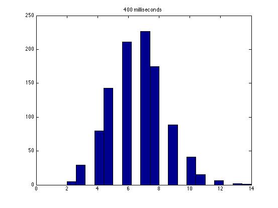
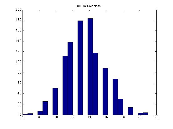
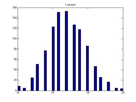
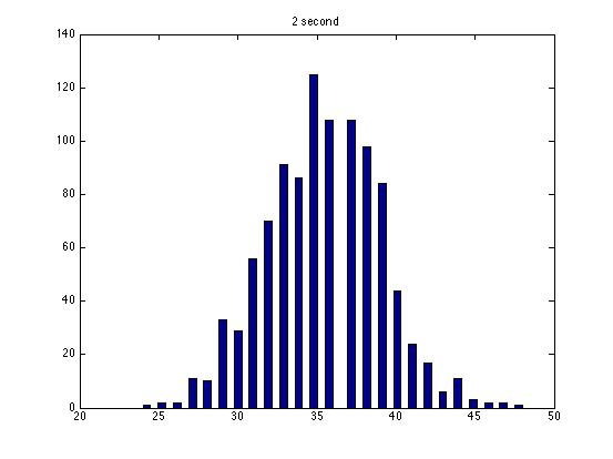
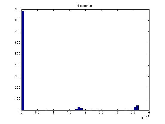
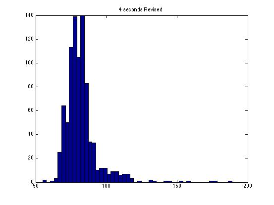
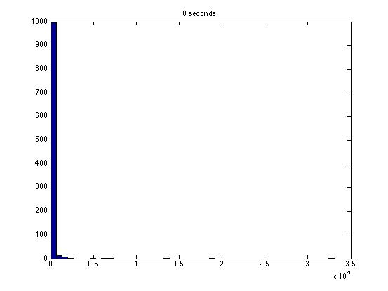
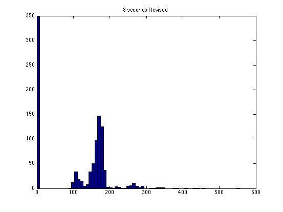
These graphs are a good start, but some things are missing. First, it would be a lot better if you could figure out how to get matlab to not put gaps of differing sizes between the bars--that makes it tough to look at the shapes of the distributions. Second, you should overlay best fit Poisson and Guassian distributions on the graph for comparison.
 |
 |
 |
|
 |
 |
| |
 |
 |
 |
|
 |
 |
|
| Dwell Time | 10 ms | 20 ms | 40 ms | 80 ms | 100 ms | 200 ms | 400 ms | 800 ms | 1 s | 2 s | 4 s | 4 s Revised* | 8 s | 8 s Revised* |
|---|---|---|---|---|---|---|---|---|---|---|---|---|---|---|
| Mean # Counts | 0.1729 | 0.3223 | 0.6523 | 1.3262 | 1.6914 | 3.2832 | 6.7139 | 13.5625 | 17.0566 | 35.4111 | 3.7427e3 | 82.3503 | 331.6879 | 171.8591 |
| σ # Counts | 0.4057 | 0.5694 | 0.7479 | 1.0653 | 1.2175 | 1.4678 | 1.8282 | 2.3434 | 2.6681 | 3.5962 | 9.8137e3 | 12.3347 | 1.6070e3 | 44.8021 |
| Square Root of Mean | 0.4158 | 0.5677 | 0.8077 | 1.1516 | 1.3005 | 1.8120 | 2.5911 | 3.6827 | 4.1300 | 5.9507 | 61.1776 | 90.7471 | 1.8212e3 | 13.1095 |
SJK 02:10, 1 November 2008 (EDT)

This is a good way to analyze the data--highlighting the fact that a Poisson distribution should have a variance equal to the mean. Thus, you noticed the mysterious fact that it does not seem like a Poisson distribution! Other groups have noticed this as well, and we still haven't solved the mystery as far as I know.
- The revised data have all anomalous readings removed. I have included analysis for original data for comparison.
The standard deviation is very close to the mean for small dwell times, but the quantities diverge for very large dwell times.
I am not entirely satisfied with these results: the standard deviations seem inaccurate for large dwell times.
If I had more time, I would compare these results with real Poisson distributions to check for consistency, and perform X2-analysis to find the probability distribution of the background radiation. I took far more sets of data than the original experiment required (12 as opposed to 3).
Charge to Mass Lab
The relevant pages of the lab notebook are 10/13/08 and 10/20/08.
In this lab, we activated a Helmholtz coil apparatus in order to measure the charge-to-mass ratio of an electron based on the deflection of an electron beam by the magnetic field generated from the Helmholtz coils, as well as the voltage used to accelerate the electron beam and the current used to generate that magnetic field.
We applied various combinations of voltages and currents until paths of electrons could be observed (left). Some of these paths glowed in the UV spectrum (center). Then the current and voltage were adjusted upward to obtain large circular paths (right), which were suitable to measure.
| Error creating thumbnail: File missing | Error creating thumbnail: File missing | Error creating thumbnail: File missing |
Using the formula (e/m) = 2*V/(B*r)^2 where
- V = accelerating voltage
- B = magnetic field strength = 7.8 * 10^4 Wb/(A m^2) * I
- I = current
- r = deflection radius,
we can calculate the following out of 12 sets of data:
| Mean Value | Standard Error of the Mean | |
|---|---|---|
| V (V) | 270.1 | 6.634 |
| B (T) | 1.059e-3 | 0.071e-3 |
| I (A) | 1.357 | 0.091 |
| r (m) | 3.5e-2 | 0.1e-2 |
| e/m |
3.829e11 | 0.335e11 |
Therefore, we can say with 68% confidence that (e/m) = 3.829 ± 0.335 * 10^11.
SJK 00:54, 3 November 2008 (EST)

You're missing units on this value (your table does have units, but you had a typo there!. You also have too many digits. Three digits on your uncertainty is unreasonably large. 3.83 +/- 0.34 or even 3.8 +/- 0.3 e11 C/kg would be easier to read and better.
We also qualitatively measured the effects of activating deflection plates in the Helmholtz coil. Applying a current to the deflection plates in the indicated direction, the electron beam is deflected upward; applying current in the opposite direction, the beam is deflected downward.
Lab Questions:
1. We see the electron beam due to the bremsstrahlung effect, which exists due to the helium in the glass tube.SJK 02:00, 3 November 2008 (EST)

Well, I have to say that you succeeded in getting me to brush up on all kinds of fun radiation that I haven't thought about in a while. I think in this case, since our electrons are far from relativistic, that the most applicable radiation due to accelration would be cyclotron radiation, and which would not be visible photons. Cerenkov radiation would also only occur for relativistic electrons making a transition into a medium with much higher index of refraction. As for bremsstrahlung effect, I think that would generally encompass cyclotron radiation. Besides knowing the electron energy (from the accelerating voltage), a piece of evidence that the visible light is not coming from bremsstrahlung effect is that the beam is colored in absence of magnetic field. Also, the distinct cyan and violet colors seen are not expected for the above effects. This is all very interesting though! The light actually comes from electrons exciting helium atoms, and then emission of visible photons as the helium atoms relax. You can see the cyan color in this helium spectrum. Now, why it's the cyan color (usually) and sometimes the violet color, I still do not understand!
2. According to the NGDC, there is an effect of roughly 23 μT. Given the magnitude of our experimental field, we can ignore this.
3. If protons were emitted, the beam would always be deflected in the opposite direction.
4. According to Wikipedia frequency f = 1/t = B * (e/m), therefore t = 1/(B * (e/m)). For constant B, time t has no dependence on V.
5. According to the equation v = rB(e/m), velocity v = 0.05021±0.00190 *c. (Mean ± Standard Error of the Mean) For such speeds v << c, relativistic corrections would not matter much.
I acknowledge this website from which I got some equations.
SJK 03:12, 3 November 2008 (EST)

Unless I am missing it, you are not comparing the magnitude of the discrepancy from the accepted value with your uncertainty from the SEM. (You probably did do this, though.) This is what tells you that you have a huge systematic error...the accepted value is very far from your 68% confidence interval.
I am not satisfied with the results. Although they are on the right order of magnitude (~10^11), they are roughly twice the accepted value of 1.76e11. Perhaps I made a calculation error, or perhaps there is a systemic error I did not identify.
If I had more time I would attempt to find the source of this error. I would also attempt to physically rotate the tube to determine the effects of deflecting the electron beam, and to further explore the effects of the Earth's magnetic field. I would also try to check my data against data taken against constant current, as well as data taken against constant voltage.
Further Analysis and Notes
SJK 00:49, 3 November 2008 (EST)

Thank you for this explanation. I now see that you calculated the e/m ratios individually and then used the mean and SEM of these values. That's sensible...as long as you didn't see any obvious trend. Did you plot the e/m ratios versus various values? For example, e/m ratio versus voltage; ratio versus current; ratio versus measurement number. If you saw a trend in any of these, then you have to really question whether the mean of all of the values is the appropriate thing to do. Of course, in this lab systematic error is such a huge factor it tends to dominate this kind of thinking.
The mean and standard error of the mean (SEM) values for voltage, current, magnetic field strength, and beam radius are included not for any intrinsic value, but because we originally believed they might have aided in the calculation of the SEM value for the charge-to-mass ratio through the principle of propagated error.
They were useful for computing the mean of the ratio. However, they were useless for the SEM since the values of voltage, current, and beam radius are not independent. As such, traditional formulas for error propagation for independent variables do not apply, and since we have all values in the computer, we can compute the SEM directly (which we ultimately did).
The mean of e/m ratios was calculated from inputting the means of the variables into the equation for e/m. The SEM of e/m was calculated from the (automatic) standard deviation function applied over each individual e/m ratio as calculated from corresponding sets of voltage, current, and beam radius, divided by the square root of the number of ratios. (All other SEM values were calculated in a similar way; the standard deviation of the set of all values, divided by the square root of the size of the data set).
The MATLAB M-file used to compute all quantities is here:
function RatioLab
format long;clc
V = [268.4 244.7 290.4 264.2 289.4 283.6 231.7 292.2 255.1 281.2];
Vmean = mean(V)
I = [1.283 1.208 1.180 1.409 2.099 1.330 1.002 1.418 1.380 1.265];
Imean = mean(I)
r = [4.0 3.5 3.8 4.2 4.0 3.6 3.9 4.1 4.6 3.6 4.5 4.7 3.7 3.5 3.0 3.3 2.0 1.7 1.8 2.0 4.1 3.5 3.9 4.1 3.9 3.6 4.1 4.4 3.6 3.4 3.3 3.5 2.7 2.5 2.6 2.9 4.3 3.8 4.0 4.2];
Bmean = 7.8e-4 * Imean
rmean = mean(r)/100
ratiomean = 2 * Vmean/((Bmean * rmean)^2) % mean
VSEM = std(V)/sqrt(length(V))
ISEM = std(I)/sqrt(length(I))
rSEM = std(r)/sqrt(length(r))
BSEM = 7.8e-4 * std(I)/sqrt(length(I))
r = [4.0 3.5 3.8 4.2;4.0 3.6 3.9 4.1;4.6 3.6 4.5 4.7 ;3.7 3.5 3.0 3.3 ;2.0 1.7 1.8 2.0 ;4.1 3.5 3.9 4.1; 3.9 3.6 4.1 4.4; 3.6 3.4 3.3 3.5 ;2.7 2.5 2.6 2.9; 4.3 3.8 4.0 4.2];
ratio = 2 .* V./(((7.8e-4 .* I) .* mean(r'/100)).^2)
ratioSEM = std(ratio)/sqrt(length(ratio)) % standard error of the mean
vel = mean(r'/100) .* (7.8e-4 .* I) .* ratio
velmean = mean(vel)
velC = velmean/3.0e8
velSEM = std(vel)/sqrt(length(vel))
velCSEM = velSEM/3.0e8
Balmer Series Lab
The raw data from the lab is on the notebook pages from 10/27/2008, 11/3/2008, and 11/16/2008.
In this lab, we observed the wavelengths of light emitted from various elemental lamps in order to determine the Rydberg constant.
First, we had to calibrate the spectrometer by shining a mercury lamp at it, and comparing the measured wavelengths with accepted values. Then we measured the visible second-order emmission spectra from regular hydrogen and deuterium lamps (also known as the "Balmer series") with the spectrometer in order to determine the Rydberg constant, as well as a krypton lamp to determine how well our equipment could resolve.
Our spectrometer seemed to be able to visibly resolve wavelengths within ~1 nm of each other and no closer. We determined this by observing the violet end of the krypton spectrum.
The value for the Rydberg constant for hydrogen was measured as 10964446.07 ± 7548.89 1/m (mean ± SEM). Compared with the official value of 10967758 1/m, we find an astonishingly low 0.0302% error (thus we note that the mean value is within one standard deviation the accepted value).
The value for the Rydberg constant for deuterium was calculated as 11055173 1/m, which has a 0.7970% difference from the Rydberg constant for hydrogen. Qualitatively, however, there is no clear difference between the spectra for regular hydrogen and deuterium.
I am satisfied with the results; I obtained a value very close to the canonical value for the Rydberg constant with multiple measurements, with small error that appears random.
Although I did not have time to calculate the precise canonical differences in second-order wavelengths from hydrogen to deuterium, I was able to take 3 sets of measurements each.
Astonishingly, all sets of measurements were extremely consistent; I obtained the same values for wavelengths on each of 3 measurements of both the hydrogen and deuterium spectra. I do not know why that is the case.
