Cameron M. Rehmani Seraji Week 4
From OpenWetWare
Jump to navigationJump to search
Cameron M. Rehmani Seraji Electronic Notebook Week 4
Purpose
- The purpose of this assignment was to model the nutrient/cell population model in MATLAB and see how changing the different state variables and parameters affected the amount of food and the amount of cells inside the chemostat.
Methods
- Week 4 Assignment PDF was referenced for the directions of this assignment.
- Created the function 'chemostatCR.m'.
function dx = chemostatCR(t,x)
global q u V K r
dx = zeros(size(x));
dx(1) = ((q*u) - (q*x(1)) - x(2)*(V*x(1))/(x(1)+K));
dx(2) = -(q*x(2))+(r*x(2))*((V*x(1))/(x(1)+K));
end
- Created the script 'chemostatCRscript.m'.
global q u V K r
q=2;
u=3;
V=10;
K=50;
r=5;
tt = 0:0.1:50;
x0 = [5;10];
[t,x] = ode45('chemostatCR',tt,x0);
plot(t,x)
xlabel('time')
ylabel('concentration')
title('Population and Food Source Over Time')
legend('Population','Food')
- Added the mortality term to 'chemostatCR.m'
function dx = chemostatCR(t,x)
global q u V K r d
dx = zeros(size(x));
dx(1) = ((q*u) - (q*x(1)) - x(2)*(V*x(1))/(x(1)+K));
dx(2) = -(q*x(2))+((r*x(2))*(V*x(1))/(x(1)+K)) - (d*x(2));
end
- Added the mortality term to 'chemostatCRscript.m'
global q u V K r d
q=2;
u=16;
V=15;
K=65;
r=5;
d=6;
tt = 0:0.1:3;
x0 = [1;2];
[t,x] = ode45('chemostatCR',tt,x0);
plot(t,x)
xlabel('time')
ylabel('abundance')
title('Population and Food Source Over Time')
legend('Population','Food')
- Added second nutrient to 'chemostatCR.m'
function dx = chemostatCR(t,x)
global q u V K r
dx = zeros(size(x));
dx(1) = ((q*u) - (q*x(1)) - x(2)*(V*x(1))/(x(1)+K));
dx(2) = -(q*x(2))+((r*x(2))*(V*x(1))/(x(1)+K));
dx(3) = ((q*u) - (q*x(3)) - x(2)*(V*x(1)+x(3))/(x(1)+x(3)+K));
end
- Added second nutrient to 'chemostatCRscript.m'
global q u V K r
q=2;
u=.66;
V=55;
K=65;
r=5;
tt = 0:0.1:3;
x0 = [1;2;3];
[t,x] = ode45('chemostatCR',tt,x0);
plot(t,x)
xlabel('time')
ylabel('abundance')
title('Population and Food Source Over Time')
legend('Population','Food')
Results
Part 1
- A. First, make sure you understand which variables are the state variables (dependent variables that determine the concentrations) and which variables are parameters (e.g., rate constants).
- The state variables are:
- Consumption rate = -yVmax(c/K+c)
- The parameters are:
- inflow rate = q*u
- outflow rate = q*c(t)
- outflow rate = -q*y
- net growth rate = r
- B. Find values of c and y that hold the system in equilibrium: that is, find values of c and y for which constant functions at those values are actually solutions of the differential equation system.
- y = 0, c = u
- C. Simulate this system with different values for the constants and the initial concentrations of nutrients and cells. The initial nutrient level can be =0, but the constants and the initial cell population size need to be positive. Can you make any observations about how the system behaves?
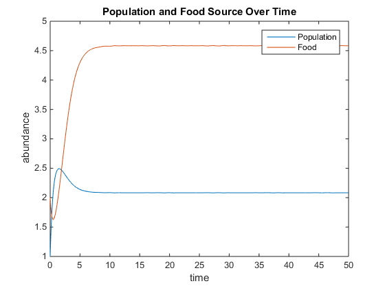
- Figure 1. In this system the different constants and initial concentrations were set at: q=2, u=3, V=10, K=50, and r=5. From looking at the graph, initially the population is greater than the amount of food, but as the population begins to drop the amount of food continues to climb. The population appears to level off around 2 and the amount of food levels off around 4.5.
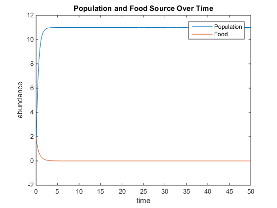
- Figure 2. The different constants and initial concentrations were set at: q=2, u=2, V=0.8, K=50, and r=5. At the start, population and food are near each other at around 2, but population grows very quickly to approximately 11 by time 5 and the amount of food goes down to 0 by time 5. The lines do not appear to change after time 5, which is strange because the population should decrease because there is no food in the chemostat.
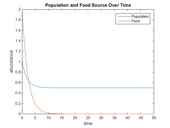
- Figure 3. The different constants and intial concentrations were set at: q=0.5, u=0.5, V=0.1, K=10, and r=5. Population and food both decrease from the very start. Food started at 2 at time 0 and had decreased to 0 by time 15. Population started at 1 at time 0 and decreased to 0.5 by time 5 and did not change for the remainder. Population should decrease to 0 because there is no food in the chemostat.
Part 2
- What changes if we return a mortality term to the population equation? Repeat b and c for a linear mortality term.
- The system will be at equilibrium at the same values.
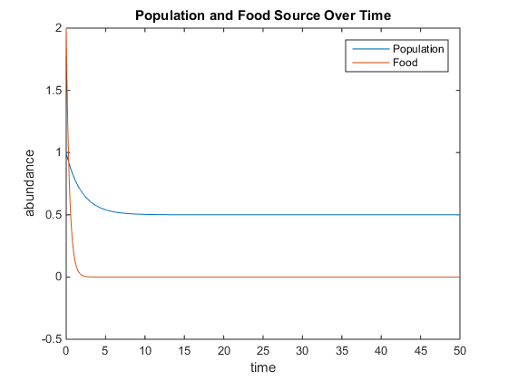
- Figure 4. The different constants and initial concentrations were set at: q=0.5, u=0.5, V=0.1, K=10, r=5, and d=6. D represents the mortality term. Adding the mortality term caused the population go down quicker than it did without it and it also caused the food supply to not decrease as much as it did without it.
![]()
- Figure 5. The different constants and initial concentrations were set at: q=2, u=16, V=15, K=65, r=5, and d=6. At the start, the population and food both start to increase until the amount of food becomes greater than the population. At time 1.5, the amount of food decreases again and will eventually level off at approximately 10.
Part 3
- Create a model with two nutrients, both of which are required for the population to grow.
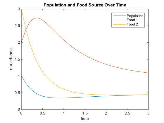
- Figure 6. A second nutrient has been added to chemostat. The different constants and initial concentrations were set at; q=2, u=0.6, V=55, K=65, and r=5.
Scientific Conclusion
- In conclusion, yeast growth was determined by the nutrient concentration, dilution rates, mortality rates, and the volume of the chemostat. The chemostat adds nutrients at a fixed rate and concentration, food flows out at a fixed rate, and the amount of food can never go below zero because it is constantly being added to the chemostat. In an ideal situation, the population can grow as much as it wants with an unlimited, constant amount of food. In all of the scenarios, the amount of nutrients and the population leveled out.
Acknowledgments
- I worked with Lauren M. Kelly, Margaret J. O'Neil, Conor Keith, and Nika Vafadari in Seaver 120. We worked on the MATLAB script and function.
- I modeled the function and script off of what Dr.Fitzpatrick showed us how to do in class.
- Except for what is noted above, this individual journal entry was completed by me and not copied from another source.
- Cameron M. Rehmani Seraji 23:14, 8 February 2017 (EST):
References
- Dahlquist, Kam D. (2017) BIOL398-05/S17:Week 4. Retrieved from http://www.openwetware.org/wiki/BIOL398-05/S17:Week_4 on 8 February 2017.
Navigation Links
- Cameron M. Rehmani Seraji
- Weekly Journal Entries
- Cameron M. Rehmani Seraji Week 2
- Cameron M. Rehmani Seraji Week 3
- Cameron M. Rehmani Seraji Week 4
- Cameron M. Rehmani Seraji Week 5
- Cameron M. Rehmani Seraji Week 6
- Cameron M. Rehmani Seraji Week 7
- Cameron M. Rehmani Seraji Week 7 Redo
- Cameron M. Rehmani Seraji Week 9
- Cameron M. Rehmani Seraji Week 10
- Cameron M. Rehmani Seraji Week 11
- Cameron M. Rehmani Seraji Week 12
- Cameron M. Rehmani Seraji Week 14/15
- Weekly Assignment Pages
- Shared Journal Pages
- Template:Cameron M. Rehmani Seraji
