Cameron M. Rehmani Seraji Week 2
From OpenWetWare
Jump to navigationJump to search
Cameron M. Rehmani Seraji Electronic Notebook
Purpose
- The purpose of the Week 2 Assignment was to practice using the functions of MatLab, create a script of two vectors and plot them, and to create a script to compare logistic growth curves.
Methods
- Part I: Create a script that includes the following elements
- Define a vector u containing the elements 1,2,3,4,5,6,7,8,9,10 using the colon operation.
- u=[1:10]
- Define another vector v containing elements that are the square of the vector x
- v=u.^2
- Plot v versus u (make sure you know what that sentence means!!) using circles on the points that are connected with dashed lines
- plot(u,v)
- Save your plot as a TIFF file
- Save your data into an excel spreadsheet using the MATLAB command xlswrite
- Define a vector u containing the elements 1,2,3,4,5,6,7,8,9,10 using the colon operation.
- Part II: Create a script to compare logistic growth curves
- Define a vector t starting at 0, ending at 1, in steps of 0.01.
- t=[0:0.01:1]
- Define K = 10 and x0 = 2 for carrying capacity and initial population size.
- K=10. x0=2
- Plot logistic growth curves for growth rates 0.5,1.0,1.5, and 2.0.
- y1=(x0*K)./(K*exp(-0.5*t)-x0*exp(-0.5*t)+x0)
- y2=(x0*K)./(K*exp(-1.0*t)-x0*exp(-1.0*t)+x0)
- y3=(x0*K)./(K*exp(-1.5*t)-x0*exp(-1.5*t)+x0)
- y4=(x0*K)./(K*exp(-2.0*t)-x0*exp(-2.0*t)+x0)
- Plot these four curves together in one figure, and add appropriate labels, title, and legend.
- Save your plot as a TIFF file
- Define a vector t starting at 0, ending at 1, in steps of 0.01.
Results
Part 1

- Figure 1: Display of the relationships between vector U and vector V.
Vector U (Row 1) and Vector V (Row 2) Data
Part 2
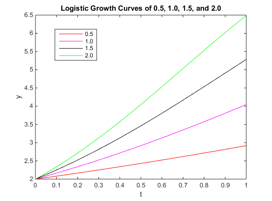
- Figure 2: Logistic growth curves for r=0.5,1.0,1.5, and 2.0.
Scientific Conclusion
- The scientific conclusion from the week two assignment is that linear growth curves grow more rapidly as the r value increases and I completed the purpose by plotting u versus v and plotting the four logistic growth curves on the same figure. These curves are shown above.
Acknowledgements
- I worked with my homework partner Lauren M. Kelly face-to-face in the Seaver computer lab outside of normal class hours. We worked on the MATLAB portion of the assignment together.
- Except for what is noted above, this individual journal entry was completed by me and not copied from another source.
- Cameron M. Rehmani Seraji 01:23, 26 January 2017 (EST):
References
Navigation Links
- Cameron M. Rehmani Seraji
- Weekly Journal Entries
- Cameron M. Rehmani Seraji Week 2
- Cameron M. Rehmani Seraji Week 3
- Cameron M. Rehmani Seraji Week 4
- Cameron M. Rehmani Seraji Week 5
- Cameron M. Rehmani Seraji Week 6
- Cameron M. Rehmani Seraji Week 7
- Cameron M. Rehmani Seraji Week 7 Redo
- Cameron M. Rehmani Seraji Week 9
- Cameron M. Rehmani Seraji Week 10
- Cameron M. Rehmani Seraji Week 11
- Cameron M. Rehmani Seraji Week 12
- Cameron M. Rehmani Seraji Week 14/15
- Weekly Assignment Pages
- Shared Journal Pages
- Template:Cameron M. Rehmani Seraji
