BISC 111/113:Lab 2: Population Growth
Objectives
1. To set up a student designed experiment on the factors affecting population dynamics in a species of flour beetles, Tribolium confusum.
2. To learn how to use the computer program Excel for graph construction and the computer program JMP for statistical tests.
Lab 2 Overview
I. Formulate experimental questions and hypotheses about population growth of Tribolium
- II. Design and set up tests of your population growth hypotheses
- a. Post a PowerPoint summary of your experimental design
-
III. Data Analysis and Presentation
- a. Learn how to calculate the mean, variance, standard deviation, and standard error of data arrays
- b. Learn how to test for differences in the means of two samples using the t-test.
Population Growth Background
It is accepted that environments on Earth are finite and therefore have limited resources, so it follows that no population can grow indefinitely. Certainly no organism exhibits its full reproductive potential. Darwin, for example, calculated that it would take only 750 years for a single mating pair of elephants (a species with a relatively low reproductive potential) to produce a population of 19 million. This is vastly in excess of the current total population and elephants have existed for millions of years. Some species might exhibit population explosions for a short time (e. g., algal blooms), but their population inevitably crashes. Most populations, however, are relatively stable over time, once they have reached an equilibrium level.
Population ecology is the discipline that studies changes in population size and composition, and also tries to identify the causes of any observed fluctuations. A population is made up of interbreeding individuals of one species that simultaneously occupy the same general area. Fluctuations in population sizes could be caused by environmental conditions as well as by predation, disease, and interspecific competition. It can be particularly challenging to follow and understand the population dynamics of a species in the "real" world. Therefore, scientists have often used controlled lab experiments to understand the basic concepts of population ecology. Many classical experiments have explored population dynamics of and inter- and intraspecific competition in the flour beetles, all members of the genus Tribolium.
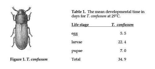
While Tribolium can survive on a number of finely ground grains, these particular beetles are cultured in 95% whole wheat flour and 5% brewer's yeast. Tribolium thrive at a temperature range of 29-34 °C and a humidity of 50-70%. Under optimum conditions one would expect a new generation roughly every 4 weeks (Table 1, from Park, T., 1948, Experimental studies on interspecies competition Ecological Monographs, 18, 267-306). The "confused" flour beetle (T. confusum) (Fig. 1) was so named because it was often confused with its closely allied species T. castaneum.

Because a female flour beetle can live at least a year and lay 400-600 eggs in her lifetime, one can imagine the potential for overcrowding. High density can lead to several interesting phenomena, such as an increase in the incidence of cannibalism, where the adult beetles will eat the eggs; larvae will eat eggs, pupae, and other larvae. If conditions are crowded and stressful the beetles will often produce a gas containing certain quinones that can cause the appearance of aberrant forms of young or can even kill the entire colony. There have also been reports that overcrowding leads to an increase in the transmission of a protozoan parasite (Adelina tribolii).
Arthropods need to molt in order to grow. Tribolium beetles, like all other members of the insect order Coleoptera, undergo complete metamorphosis, passing through four distinct phases to complete their life cycle: egg, larva, pupa, and adult. An egg is laid from which hatches a larva. This larva molts into a second and then third larval stage (or instar) increasing in size in the process. The third instar turns into a pupa from which finally an adult is released. The pupa is a quiescent stage during which larval tissues and organs are reorganized into adult ones.
Setting up the Experiment
Your charge is to set up an experiment dealing with population ecology of the flour beetle. You should start your experiment with at least 20 beetles per container, because they are not sexed. This should ensure enough females in your starting population. We have found that 1 gram of food per beetle will keep them reasonably healthy until the end of the experiment. Discuss the appropriate number of replicates and what conditions you will set as your control.
Some of the factors you could consider investigating are:
Size of starting populations (intraspecific competition)
Food supply (e.g., various milled flours, whole grains, prepared grain products, and/or brewer's yeast)
Environmental structure (effects of environmental patchiness on population growth, e.g., habitat size, light availability, refuge use, or "dilution" of the food/habitat volume with inert materials)
Biological control of populations in grain storage facilities (e.g., diatomaceous earth, application of plant volatiles)
Briefly outline the hypothesis that you are testing or your experimental question in your lab notebook. Provide details of your experimental design (starting number of beetles, number of replicates, variables, etc.)
With your group, prepare a PowerPoint slide(s) describing the goals and design of your Tribolium experiment and post it to Sakai. This set of PowerPoint slides will serve as an outline for the Materials and Methods section of the paper you will write on your beetle experiment at the end of the semester. Thus, you should be sure to include the details of your design today, including a description of each variable condition, number of replicates, number of beetles per jar, food type/quantity, conditions of the environmental chamber, and any other information you feel would be important to include in your Materials and Methods section. It may help you to review the section about Materials and Methods in the Science Writing Guidelines to make sure you include the necessary information.
Descriptive Statistics
When dealing with the dynamics of populations, whether they are beetles in a jar or plants in the field, we infer population-level characteristics from small portions, or samples, of the population. Otherwise the task could be overwhelming. As scientists, our inference of population behavior is based on the assumption that the selected members of the population were randomly sampled. Random sampling means that the likelihood of any particular individual being in the sample is the same for all individuals, and that these individuals are selected independently from one another. A statistical test is the impartial judge of whether our inferences about the at-large population(s) are sufficiently supported by our sample results. See Statistics and Graphing for tutorials for calculating all of the statistics below with Excel 2008 and JMP.
Descriptive statistics are measures of location and variability used to characterize data arrays. In this course, we will use hand calculation and the computer programs Excel and JMP to generate common descriptive statistics.
Statistics of location are measures of "location" or "central tendency."
The mean, median, and mode are all measures of location. The mean is the most commonly used of these, and estimates the true population mean if it is based on samples composed randomly from the at-large population. Calculate the mean of a data set by dividing the sum of the observations by the number of observations.
Statistics of variability provide estimates of how measurements are scattered around a mean or other measures of location. Both biological variability and the accuracy of our measurements are sources of variability in our data.
Variance is an approximate average of the square of the differences of each value from the mean. However, because the variance is reported as the square of the original unit, interpretation can sometimes be difficult. The variance of a sample is calculated by taking the sum of the squared differences between each value and the mean value, divided by the number of observations less 1 (when based on a random sample from the population).
Standard Deviation (SD) is a common measure of variability that avoids the problem of units inherent in the variance. The standard deviation is calculated by first calculating the variance, and then by taking its square root.
Standard Error of the Mean (SEM or SE) estimates the variation among the means of samples similarly composed from the population at large (the so-called "true" population). The SE estimates the variability among means if you were to take repeated random samples of the same size from the population. A small SE indicates that the sample mean is close to the true population mean. With increasing sample sizes (n) the SE shrinks in magnitude. Calculate the SE by dividing the SD by the square root of n.
Comparative Statistics
Comparative Statistics are ways of evaluating the similarities and/or differences among different data sets. Many situations arise in experimental and observational research where we wish to compare two outcomes or contrasts, such as a control vs. a treatment effect.
The t-test compares the means of two samples. If the samples are taken from the same experimental unit at different times, the test is termed "paired," so a paired t-test is run. If the samples are from two different experimental units or treatments, the unpaired t-test is run. Both tests assume that data are normally distributed (i.e., have a typical bell-shaped distribution) and have equal variances. Violations of such assumptions in this kind of statistical testing are not too serious unless quite exaggerated, and there are ways to transform the data that can often rectify such problems.
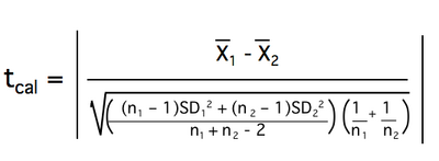
The t-test calculates a factor called the tcal by using the means, SDs, and the number of data points in each sample. Sometimes when calculated digitally, it is designated the tstat. The numerator of the tcal is a measure of the difference between the means of the samples; its denominator is a measure of the standard error of the difference (using the pooled variance), which takes sample size into account. The order in which you enter the means will determine the sign of your tcal, but this does not affect its interpretation. Always report the absolute value of tcal.
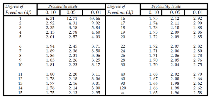
The typical null hypothesis (Ho) of a comparative statistical test is that there is no difference between the means of the populations from which the samples were drawn. Our sample means are estimators of these population means. In other words, if Ho is true, this is as if we actually drew our samples from the same population, and that any difference between our sample means is due simply to random sampling error (i.e., by chance alone). Therefore, if a significant difference is seen, the null hypothesis is rejected, meaning that our samples likely represent different populations. To determine whether two means are significantly different one must compare the absolute value of tcal to the tabulated t-value, ttab. The ttab values (and those for any other tabulated statistic) are all calculated under the null hypothesis; i.e., they represent values assuming Ho is correct. A subset of ttab values for given degrees of freedom can be found in the table below. "Degrees of freedom" (df) is based on sample size; the larger the sample size, the more "freedom" you have to make decisions about statistical significance. For a two-sample t-test, the t-statistic has df equal to the sum of the two sample sizes (n1 + n2), minus 2. The probability that a difference at least as big as the one you observed could have occurred through random sampling error alone can be read from the "Probability Levels" columns. Generally, if the probability level (P-value) of our tcal is ≤ 0.05, we can claim that there is a significant difference between the two means; that indeed, the conclusion that the two samples represent different populations, or that there was a treatment effect, is supported by our results. We would deem the null hypothesis unlikely to be true. Note that there is still the risk (1 in 20 for the probability, or significance, level of 0.05) that we would be wrong. (In fact, if our criterion to claim significance is set at P ≤ 0.05 and we were to repeat such an experiment many times, 1 in 20 times on average we would wrongly reject the null hypothesis.) But this is a risk we generally consider acceptable. In some studies, we set the bar of significance even “higher” (by lowering the P-value at which we would reject the null hypothesis and claim a significant difference between means). Occasionally, this threshold P-value (also called the alpha [α] level, below which we will claim a significant difference or effect) might be set higher (e.g., α = 0.10), but this usually needs a vigorous defense by the researcher.

Table 2. Critical tabulated values of Student's t –test (two-tailed) at different degrees of freedom and probability level
Assignments
- With your research team, prepare a group PowerPoint on the beetle experiment you designed and implemented today. Upload on Sakai before leaving lab.
- Make a column graph of Tribolium means ± SD with caption from a historical dataset (refer to your instructors assignment). In a separate paragraph, analyze your results. Present the statistical information as directed by your lab instructor. See the Statistics and Graphing tutorials for directions that will help you make a column graph of means ± SD and perform the appropriate statistical tests. See the Science Writing Guidelines for results section guidelines and examples of proper figure formatting.
- With your bench mates, prepare a summary (as described by your instructor) of the key characteristics of your plant to be presented at the beginning of lab next week.
- In preparation for the Plant Biology series, consider visiting the College Greenhouse, paying particular attention to the different adaptations of plants located in the Desert, Tropical, Subtropical and Water Plant rooms. Use the Greenhouse Map and Self-Guided Tour information.
- Take Pre-Lab quiz prior to the next lab.


