Asymmetries in Flow - Sara Koprek
Fundamentals of Mixing
Mixing can be described as a physical process through which two or more components are combined in a way such that a uniform distribution is achieved; it is a fundamental unit operation that is needed for a variety of applications. However, due to differences in macroscale and microscale flow phenomenon, mixing occurs differently, and hence, the design and implementation of mixers also differs greatly between these two systems. To understand the forces that govern the respective systems and contribute to mixing, there are several key dimensionless numbers and mathematical relationships to be considered.
Diffusion and Advection

The mixing of components primarily occurs through two different phenomena: diffusion and advection. Diffusion is the process through which individual molecules move via random (Brownian) motion. This can be described by Fick's first law,
[math]\displaystyle{ J = - D \nabla c }[/math]
where [math]\displaystyle{ J }[/math] is the flux, [math]\displaystyle{ D }[/math] is the diffusivity of the respective species, and [math]\displaystyle{ \nabla c }[/math] is the concentration gradient, which serves as the driving force of the process. If two species with different concentrations are contained in an isolated environment, molecules from each species will diffuse into the other until the overall concentration becomes uniform; it is at this point where the species are effectively mixed. The time required for mixing to occur, the mixing time ([math]\displaystyle{ t_{mix} }[/math]), is dependent on the diffusivity ([math]\displaystyle{ D }[/math]) of the species and the length over which diffusion must occur, which is known as the striation length ([math]\displaystyle{ l_{st} }[/math]). [1] The mixing time can be expressed by the following equation.
[math]\displaystyle{ t_{mix} }[/math] ~ [math]\displaystyle{ \frac {{l_{st}}^2}{D} }[/math]
Based on this relationship, it is evident that decreasing the striation length is necessary for decreasing the mixing time, which can be seen in Figure 1. [1] This idea leads into the fundamental concepts of mixing: decreasing the distance over which diffusion must occur and the process of diffusion itself.
In contrast to diffusion, advection is the process through which molecules move via the movement of the bulk, otherwise known as flow. Compared to diffusion, advective mixing is much faster and much more efficient. The degree of diffusive and advective mixing that takes place is dependent on the type of fluid flow, which can be characterized by the Reynolds number (Re).

The Reynolds number (Re) is defined as the ratio between inertial and viscous forces, and it is used to define the flow regime of a fluid. At low Reynolds number (Re < 2300), viscous forces dominate over inertial forces; these viscous forces dampen any disturbances in the flow, and as a result, the fluid moves in a smooth, layered fashion through the channel. [2] This type of flow is known as laminar flow. At high Reynolds number (Re > 4000), inertial forces dominate over viscous forces; in this case, the fluid has enough kinetic energy to overcome the damping viscous forces, meaning that any disturbances in the flow propogate, resulting in turbulent flow. [2] The differences between these two flow regimes are shown in Figure 2.
At the macroscale, fluids can take on a variety of flow regimes. By altering the characteristic length of a channel or increasing the linear velocity, the Reynolds number (Re) can be increased, and the flow can be made turbulent. This turbulence or irregularity in the flow is one of the driving forces for advective mixing.
At the microscale, the characteristic length is particularly small, resulting in Reynolds number (Re) between 0.01 and 100, restricting the flow to the laminar flow regime. [2] The parallel streamlines of the fluid means that no advective mixing can occur, and instead, only diffusion can occur between the parallel streams. Therefore, microfluidic systems are solely dependent on diffusive mixing. This is further illustrated by the Péclet number (Pe).
The Péclet number (Pe) is a dimensionless number that describes the ratio between advective and diffusive forces, and it is also used to describe the ratio between advective and diffusive timescales. The Péclet number (Pe) is defined as:
[math]\displaystyle{ Pe = \frac{(Advection \, rate)}{(Diffusion \, rate)} = \frac {t_{diff}}{t_{adv}} = \frac {L^2/D}{L/U} = \frac {UL}{D} }[/math]
where [math]\displaystyle{ U }[/math] represents the linear velocity, [math]\displaystyle{ L }[/math] represents the length scale of the flow, [math]\displaystyle{ D }[/math] represents the mass diffusion coefficient, [math]\displaystyle{ t_{diff} }[/math] represents the characteristic time for diffusion, and [math]\displaystyle{ t_{adv} }[/math] represents the characteristic time for advection. [1]
In the case of microfluidic devices, where mixing relies solely on diffusion, the time for mixing to occur can be defined as:
[math]\displaystyle{ t_{mix} = t_{diff} = t_{conv} Pe }[/math].
Therefore, the length required for mixing to occur can be defined as:
[math]\displaystyle{ L_{mix} = U t_{mix} = L Pe }[/math].
The linear relationship between the mixing time and the Péclet number (Pe) therefore suggests that the channel length required for mixing to occur increases linearly with the flow velocity. [1] This length to achieve to mixing via diffusion only can become excessively long (>> 1 cm). Thus, it is necessary to incorporate different mixing schemes such that the mixing time becomes less dependent on the Péclet number (Pe) in order to prevent excessively long channels.
In many microfluidic devices, the Reynolds number (Re) is particularly small, where Re << 1. This results in a special kind of laminar flow, where the inertial effects are considered to be negligible and only viscous forces apply. This type of flow is called Stokes flow or creeping flow. Stokes flow is described by Stokes equation, which is a simplified form of the Navier-Stokes equation. The Navier-Stokes equation for an incompressible fluid describes the motion of a Newtonian fluid by taking under consideration the conservation of momentum, the conservation of mass, the density of the fluid ([math]\displaystyle{ \rho }[/math]), pressure ([math]\displaystyle{ p }[/math]), and gravity ([math]\displaystyle{ g }[/math]). The Navier-Stokes equation for an incompressible fluid is shown in Figure 3.
-
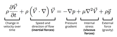
Figure 3. Navier-Stokes equation for incompressible flow with labelled components. 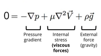
Figure 4. Stokes equation for incompressible flow with labelled components.


After neglecting the interial terms, the left hand side disappears, and the nonlinear, time-dependent Navier-Stokes equation becomes time-independent and linear with respect to velocity, as shown in Figure 4. Without the dependence on time, the previous history of the flow is not needed to understand the current state of the flow. This means that the behavior of the flow can be predicted simply by knowing the current conditions. Thereby, Stokes flow is considered instantaneous. The instanteity of the flow results in reversibility of the flow. [3] For example, imagine some fluid flowing through a channel. The moment a new set of boundary conditions is applied, the flow adjusts accordingly, due to the instanteity. If the reverse or opposite boundary conditions are then applied, the flow will adjust again and return to its initial state.
A popular demonstration of the reversibility of Stokes flow is the Taylor-Couette experiment, shown in Figure 5. In the Taylor-Couette experiment, dye is injected into a highly viscous fluid that is trapped between two cylinders. When the one of the cylinders is rotated, thereby changing the boundary conditions, the dye moves accordingly (Stokes flow). When the cylinder is rotated back to the starting position, the dye also returns to its initial state, illustrating how Stokes flow is reversible. Therefore, when designing mixers for microfluidic flow, avoiding symmetry is necessary for ensuring mixing occurs.
Microfluidic Mixing
Thus far, several phenomena and mathematical relationships regarding microfluidic mixing have been discussed, and several key points have been developed.
- The amount of time for diffusion to occur is based on the striation length.
- Microfluidic flow is restricted to the laminar region, hence, mixing can only occur through diffusion.
- For microfluidic devices, the length of the channel needed for mixing linearly increases with the velocity of the fluid.
- Since much of microfluidic flow is Stokes flow, the flow is reversible.
Based on these principles, strategies to decrease the striation length, decrease the required channel channel length, and minimize symmetry must be employed in order to efficiently mix fluids in microfluidic channels. These criteria can be met via the principle of chaotic advection.
Chaotic Advection
Mixing is a complex phenomena that is not entirely understood, but it can be described as the continuous stretching and folding or breaking and rejoining of fluids. [4] A physical representation of this transformation is mixing play-doh. Suppose you want to mix two different colors of play-doh together, the best way to do so is to stretch and recombine the play-doh over and over again until the colors are perfectly mixed. This continuous stretching and folding of fluids is known as chaotic mixing or chaotic advection. In this case, the term chaotic means that the flow is sensitive to its initial conditions, and that there is an exponential growth of fluid filaments. [4]
One mathematical explanation of this type of mixing is known as Baker’s transformation, a simple dynamical systems theory. Baker's transformation consists of stretching, cutting, and then rejoining such that the striation length decreases uniformly. Each time the transformation is applied, the striation length decreases by a factor of two, resulting in an exponential decrease in striation length. [1] As a result of decreasing the striation length, the interfacial surface area increases, and thus mixing through diffusion occurs faster. A schematic of Baker's transformation is shown in Figure 6. The time required for mixing to occur can be explained by the following equation, where [math]\displaystyle{ t_{mix} }[/math] is the mixing time and [math]\displaystyle{ t_{adv} }[/math] is time required to transvere one unit of the mixer.
[math]\displaystyle{ t_{mix} }[/math] ~ [math]\displaystyle{ t_{adv} \, log \, Pe }[/math]
As a result of chaotic advection, the mixing time only scales logarithmically with the Péclet number instead of linearly with the Péclet, showing that chaotic advection is much more effective than pure diffusion. [1]
As illustrated, chaotic advection is effective at promoting mixing; however, in order for chaotic advection to occur, the flow must have three degrees of freedom. [1] A steady, bounded, two-dimensional flow only has two degrees of freedom, as the constraints of the system generate symmetric flow; this is exhibited by the streamlines aligned in a parallel fashion (laminar flow). [4] This means that fluid is flowing through a straight mircofluidic channel cannot experience chaotic advection, as chaotic advection requires streamline crossing or asymmetry in the flow. [4] However, through the addition of a third dimension, chaotic advection can be induced. One way is through implementing 3D flow with periodicity in space. More importantly, however, if 2D flow is made to be periodic in time, the three degrees of freedom criteria is met. [4] Through the addition of an additional dimension, alternating flow patterns can be generated, which causes periodic velocity that results in chaotic mixing. [5]
It is important to note that despite the stretching and folding of the fluid and the lack of parallel streamlines, the flow still has a low Reynolds number, and it is still considered laminar flow.
Microfluidic Mixers
In order to induce chaotic advection, and therefore effective mixing, in microfluidic devices, several methods have been developed which harness the concept of inducing asymmetrical flow.
In one instance, Stroock et al. fabricated ridges on the bottom of the channel at oblique angles in order to induce transverse flows and therefore induce chaotic advection. [6] The ridges are described to be similar to the rifling in a gun barrel, which present anisotropic resistance to the viscous flow. When the fluid flows parallel to the oblique valleys and peaks, the fluid experiences less resistance than flowing straight through the channel, which is orthogonal to the ridges. These ridges result in tranverse flows, which strech and fold volumes of fluid over the cross section of the channel, ciruculating through the channel. Stroock et al. termed the patterned groves "staggered herringbone mixers" (SHM), in which the asymmetric groove shapes change along the channel. [6] Compared to simple diagnol grooves, these staggered herringbone mixers provide much greater mixing. By changing the orientation of the herringbones every half cycle, the centers of rotation change, resulting in counter-rotating fluid flows, leading to exponential stretching and folding, and thereby further decreasing the striation length and improving mixing.
In another instance, Bringer et al. were able to induce chaotic advection mixing within droplets. [7] Within a stream of immiscible fluid, they generated fluid plugs and investigated how the geometry of the channel affected mixing. When the plugs flowed through a straight channel, they found that the effectiveness of mixing inside of the plug was sensitive to initial distribution of reagents inside of the plug. Meaning that proper distribution of reagents was essential to achieving good mixing. When the plugs flowed through a winding channel, the shearing interaction between the fluid and the walls resulted in periodic recirculation of reagents and thus chaotic advection. Through chaotic advection, they were able to achieve better mixing.
The techniques mentioned are only two of many techniques capable of inducing effective mixing in microfluidic devices.
References
- Kim, S.-G.; Karnik, R.; Kim, J.; Kole, M.; Comeau, B.; Herrick, D. C. Micro/Nano Engineering Laboratory: Microfluidic Mixing https://ocw.mit.edu/courses/2-674-micro-nano-engineering-laboratory-spring-2016/resources/mit2_674s16_microfluidcmix/ (accessed 2022-05-05).
- Squires, T. M.; Quake, S. R. Microfluidics: Fluid Physics at the Nanoliter Scale. Rev. Mod. Phys. 2005, 77 (3), 977–1026. https://doi.org/10.1103/revmodphys.77.977.
- Ouldridge, T. Low Reynolds Number Hydrodynamics: Stokes’ Flow. https://www.imperial.ac.uk/media/imperial-college/research-centres-and-groups/principles-of-biomolecular-systems/Stokes_flow.pdf (accessed 2022-05-05).
- Ottino, J. M.; Muzzio, F. J.; Tjahjadi, M.; Franjione, J. G.; Jana, S. C.; Kusch, H. A. Chaos, Symmetry, and Self-Similarity: Exploiting Order and Disorder in Mixing Processes. Science 1992, 257 (5071), 754–760. https://doi.org/10.1126/science.257.5071.754.
- Ward, K.; Fan, Z. H. Mixing in Microfluidic Devices and Enhancement Methods. J. Micromech. Microeng. 2015, 25 (9), 094001. https://doi.org/10.1088/0960-1317/25/9/094001.
- Stroock, A. D.; Dertinger, S. K. W.; Ajdari, A.; Mezic, I.; Stone, H. A.; Whitesides, G. M. Chaotic Mixer for Microchannels. Science 2002, 295 (5555), 647–651. https://doi.org/10.1126/science.1066238.
- Bringer, M. R.; Gerdts, C. J.; Song, H.; Tice, J. D.; Ismagilov, R. F. Microfluidic Systems for Chemical Kinetics That Rely on Chaotic Mixing in Droplets. Philos. Trans. A Math. Phys. Eng. Sci. 2004, 362 (1818), 1087–1104. https://doi.org/10.1098/rsta.2003.1364.
