RAVE:ravepreprocess
| Reproducible Analysis and Visualization of iEEG RAVE |
Overview
To load your data into RAVE, the following items are required:
- iEEG data
- MRI data (volumetric or FreeSurfer) for visualizing anatomical locations of electrodes
RAVE can assist with generating two additional requirements:
- list of electrode labels and co-ordinates, generated from a post-implantation CT scan
- list of event times and labels, generated during the experimental session (e.g. t = 2 sec Event type 1 started; t = 3 sec Event type 1 stopped; t = 14 sec Event type 2 started; t = 16 sec Event type 2 stopped; etc.)
Preparing data
RAVE natively supports several data formats.
- BlackRock NSP files (".CCF", ".NEV", ".NSx" where x is 1-6)
- Matlab (".mat") or HDF5 (".h5") files, either:
- One file per electrode (raw voltage over time)
- One file with data from all electrodes stored in one matrix (raw voltage by electrode by time)
To grant RAVE access to your data, please copy your data into the RAVE raw-data directory. By default it is located at your home directory, under "rave_data > raw_dir" folder (if you cannot find it, expand the "Common questions" below and check question 3).
Under the raw-data directory, create a folder for your subject. The folder name needs to be consistent with the subject code (for example, "subj01")
Go to the subject folder, create a folder for each session block, copy your block voltage data respectively.
For example, suppose you have a subject (with patient code "subj01"). The subject has 5 blocks ("run01", "run02", ... "run05"). To allow RAVE to import those data, you need to go to the raw folder under "~/rave_data/raw_dir"; create folder "subj01"; enter the subject folder "subj01", create folder "run01", copy the voltage data for the first block into folder "run01"; repeat the above process for all other blocks until datasets are copied.
For more details, see RAVE's directory and file structure.
- What is a block in RAVE?
A block refers to one continuous recording session, usually one run of recording, or a task.
- What are the .NEV/.NSx files?
They are raw data from BlackRock NSP amplifiers. Some other manufacturers also use this format. For more information about this file formats, consult the amplifier manufacturer, e.g. https://github.com/BlackrockNeurotech/NPMK
- Where can I find RAVE raw-data directory?
By default, this folder is under your home directory.
For windows users, it's under
C:\Users\⟨your username⟩\rave_data\raw_dir
For Mac users, it's under
/Users/⟨your username⟩/rave_data/raw_dir
For Linux users, it's
/home/⟨your username⟩/rave_data/raw_dir
If you have altered the directory path, or not sure if you have done so, run the following R command:
raveio::raveio_getopt("raw_data_dir")
#> [1] "/Users/beauchamplab/rave_data/raw_dir"
- I have two BlackRock .NEV files in the same block, does RAVE support importing them natively?
When there are multiple NSP banks, the signals might not be synchronized across different recording devices, and you probably want to synchronize them by yourself before importing to RAVE.
However, you can convert BlackRock files to Matlab data files using the following command:
raveio::convert_blackrock("path to BlackRock .NEV or .NSx file", subject = "my subject code")
The command will extract signals for each channel and store them under the subject's raw folder. You can edit those files easily in R or Matlab.
- My data file is not listed, can I still import my data to RAVE?
Please try your best to convert your data into the above mentioned formats. RAVE does have limited support to convert some text files (such as .txt, .csv) via the following command:
rave::rave_import_rawdata('subject_code','project_name')
This command searches for the specified project_name directory within the specified subject_code directory and copies all files found there into RAVE's directory and file structure. The script requests the sampling rate of the data during data acquisition (e.g. enter 2000 for 2 kHz sampling rate), then scans the specified directory. The user selects the data blocks corresponding to the appropriate project_name. The script determined whether the data is stored as 1 file per channel or 1 file containing all channels (for this, the file name must be exactly the same across the selected blocks.) For more information, see: Detailed tutorial on ingesting data.
Selecting data to preprocess
To begin, launch the RAVE Preprocessing Module from R or RStudio with the following command:
ravedash::start_session()
The Preprocessing Module will launch in a browser window or tab, if the browser is already opened. Select Import Signals > Native Structures from the black panel list at left.
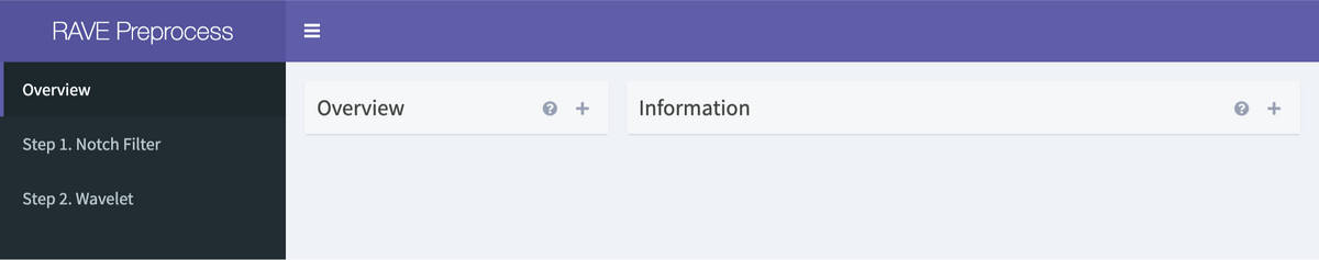
The "Native Structures" page has three sections, called panels, that contain text boxes, droplists, or checkboxes with which the files and settings for the current RAVE session are selected, or data calculated from the current panel entries. All panels have a header with the panel’s name and a minimize icon (a minus sign, “-”) that will hide the panel without altering the data therein. There may also be a help icon (a question mark, “?”), a refresh icon (a pair of circled arrows), or an expand icon (a segmented box). Those will be covered as they appear.
Look at the first panel Select project & subject. The panel has two inputs for choosing a subject’s data for preprocessing.
Step 1. Select a project folder in which to preprocess the subject data. If this is your first time using RAVE, you might want to create a new project by choosing "[New Project]" in the drop-down menu labeled Project name. Enter a meaningful project name (starts with letters) for your experiment in the pop-up dialog. If you have created the project before, simply choose the project name from the drop-down menu.
Step 2. Choose a subject code from the droplist Subject code that you want to include into the selected project. This is the name of the folder in which the subject’s raw data, where the raw iEEG recordings are stored. (In the Beauchamp lab, we use a three-letter subject code such as YAB or YAD).
RAVE automatically detects if the subject has been created before. If this is a new subject, then the button Create subject will be activated in the bottom-right of the panel. Simply click the button to initialize the subject. If the subject has been created, the button will be disabled with text Subject already exists. Please proceed to the next steps.
Look now at the second panel Format & session blocks. This panel is to select the data that will be loaded for preprocessing. In RAVE, a block refers to one continuous recording session. This could be one run/task of an experiment that lasts for minutes.
Step 3: To select the subject’s recording blocks associated with the project, choose from Sessions/Blocks menu.
Step 4: In the Formats droplist, choose a proper data format that best describe your original data.
IMPORTANT NOTE: Currently, all blocks for a subject must be preprocessed at once with the same format. This is to make sure that all blocks have the same number of electrodes and sampling rate. If additional blocks need to be added, or the format is changed later, the bottom-right button will be activated with text label Confirm, press the button to confirm changes. Please be aware that by changing the blocks or formats, the subject needs to be re-imported and re-prerocessed.
Look at the last panel Channel information. This panel is to set the electrode channels for the subject. If the data format is set correctly, there will be a small text below the drop-down menus (above the "Validate & import" button) similar to the follows:
With given data format, I found the following potential electrodes in the first block (004): 1-152,257,259
The text displays all the available channels.
Step 5: Enter the iEEG-only channels into the text input Channel numbers (in this example, 1-150 to avoid loading EKG, audio, photodiode signals)
Step 6: The rightmost input box Sample rate (Hz) sets the sample rate at which the preprocessing will be run. This should be identical to the sample rate of the iEEG recording equipment.
Leave Data file(s) and Physical unit unchanged. RAVE can to figure these out automatically.
Step 7: To import data, press Validate & import button. RAVE will validate your input, checking for potential issues such as broken data files, inconsistent data size, or missing files.
Step 8: If the validation passes, a message dialog will pop up displaying the validation results and import configurations. Please double-check the configurations. If everything is correct, press the Import button from the pop-up dialog, RAVE will start to import your signals.
Tip: a common issue is that there are some channels that you do not wish to analyze with RAVE (for instance, data from EKG leads). RAVE is designed for the case where there is a brain electrode for each channel's data stream. There are several ways to eliminate channels without associated brain electrodes. Select only the electrodes that you wish to analyze in the "Electrodes" input box (e.g. if there are 90 channels, but channels 5 through 10 are EKG channels, enter "1-4,11-90" into the input box). This will allow RAVE to skip the EKG channels. Alternately, one could make a .mat file that contains only channels 1-4 and 11-90 and then load the entire file into RAVE. Note that in this case the channel numbering will be off relative to the original channel numbering.
Click on the "?" in the menu screenshot below for more details.
Notch filtering
Click on the "?" in the menu screenshot below for more details.
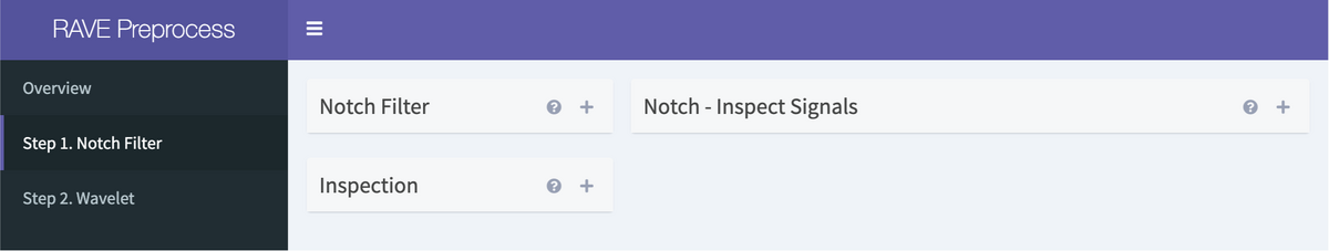
The Notch Filter is a form of band-stop filter that attenuates signals in one or a few narrow bandwidths to minimal levels while leaving signals outside the bandwidth(s) unaltered. Many iEEG setups that include an amplifier introduce harmonics at certain frequencies to the signal data. This filter removes these as a calculation of multiples of a base frequency. This panel, as well as some others seen throughout RAVE’s modules, will be autofilled with a default set of parameters; these parameters represent common settings found in iEEG and are fully customizable when encountered. The panel loads with default settings for the Notch Filter that will remove commonly-found harmonics of 60Hz introduced by most amplifiers.
First, look at the Notch Filter panel. The first text box is for the base frequency, in Hertz, of the filter. Enter here the base frequency for the notch filter. In the second text box, choose the multiplier(s) of the base frequency to be filtered out as well. The default settings are “1,2,3” and will create stopbands at 60Hz, 120Hz, and 180Hz. More multipliers can be added to cover the data’s entire frequency range if needed or, alternatively, fewer multipliers for fewer or a single stopband. The third textbox is used to set the width, in Hertz, of each stopband. One value should be entered for each harmonic, separated by commas. The default settings of “1,2,2” refer to, respectively, the 60, 120, and 180Hz bands, and refer to the +/- for each. Using the default settings, this sets the first harmonic stopband to 59-61Hz, the second to 118-122Hz, and the third to 178-182Hz. The information at the bottom of this panel will describe the number of stopbands and the ranges of each; this information will update automatically as the settings are adjusted.
Look at the Inspection panel. This panel controls the settings of the Notch – Inspect Signals panel to the immediate right which displays the raw and, after calculation, the filtered signal of each channel loaded, so these panels will be discussed together. There are two droplists side-by-side at the top of the Inspection panel. The first, to the left, controls the currently-displayed block and the second, to the right, controls the currently-displayed channel. Setting either of these will automatically update the Notch – Inspect Signals panel to display the selected recording. If it does not update automatically, click the refresh button at the top of the Notch – Inspect Signals panel. Refreshing the browser page will reset the panels to their default settings.
The “Previous” and “Next” buttons below these droplists on the Inspection panel are used to navigate between channels; pressing “Previous” will set the Notch – Inspect Signals panel to display the numerical channel immediately below the current selection, and pressing “Next” will display the channel immediately above it.
At the bottom of the Notch – Inspect Signals panel, there are two Welch periodograms and a histogram of the selected channel. Welch periodograms display the estimated power of a signal across frequencies. The rightmost plot is a standard periodogram. The middle plot is a transformation of that periodogram with a logarithmic x-axis. This makes viewing the signals at lower frequencies easier. The leftmost plot is a histogram of the voltage samples making up the displayed signal. To alter these panels, look at the three sliders at the bottom of the Inspection panel. The top slider sets the width of the Welch periodograms within the page. This will not alter the data, solely the display size of the plots within the Notch – Inspect Signals panel. The middle slider sets the frequency range of the periodograms. Frequencies outside of this range are not excluded from analysis, only from the display; the maximum frequency of the data itself is set by the recording parameters of the iEEG setting. The bottom slider controls the number of bins in the histogram. Each of these sliders can be adjusted by channel to best fit the display settings to the current signal.
Wavelet decomposition
Click on the "?" in the menu screenshot below for more details.
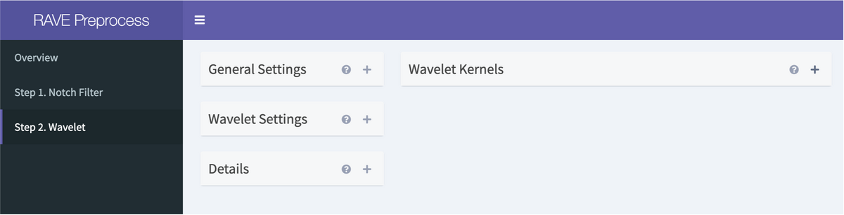
First look at the General Settings panel on the upper left. This panel has three textboxes. In the uppermost textbox labeled “Electrodes,” enter the range of the electrodes to be transformed. It’s recommended to run the wavelet across all electrodes at the same time for both consistency and best performance, so the value entered here should be “1-max” up to the largest numerical electrode value.
The wavelet is run at a native sample rate, by default 100Hz, before being down-sampled. For a different target sample rate, enter the desired value in Hertz into the second textbox.
The settings of every wavelet run are stored as a CSV file within each subject’s folder within the project. The droplist here can be used to select a previously-run wavelet setting file to repeat the transformation with the same parameters. If the desired file isn’t listed automatically in the droplist, click the “Browse” button to open a directory navigator and select the appropriate file. At the bottom of the panel is the “Run Wavelet” button that will begin the wavelet transformation. Because this process is so demanding, a dialogue box will pop up to confirm this choice. Click “Yes” if the computer is ready to run the transformation or “No” to close the dialogue box and continue editing the settings.
The Details panel does not alter the settings of the wavelet but rather displays them as a table for review. This panel will update automatically if information in the General Settings panel is changed or if a CSV file is loaded through the Wavelet Settings panel. At the top of the panel is a small blue link, “Download Current Setting.” Clicking this will download the table as a CSV to the local computer. This file is also saved automatically upon completion of the wavelet to the subject’s /meta/ folder within a project in the RAVE directory.
The Wavelet Kernels panel is the largest panel of the Wavelet page and displays graphically the details of the wavelet transformation that will be run.
Troubleshooting: If Wavelet decomposition crashes, it is often because the "Number of Cores" setting is too high. Using more CPU cores speeds up processing but also requires more RAM. Try decreasing the "Number of Cores" setting. This setting is available in the third textbox. Because the wavelet transformation requires a large amount of RAM, it must be run in parallel across multiple cores to avoid a memory shortage. The maximum number of cores and the RAM per core available to RAVE are set in the RAVE options menu, accessible by the command:
rave_options()
Epoching
Import imaging data and localize electrodes
Guide to importing imaging data and localize electrodes in RAVE
