RAVE:Tutorial Clusters

Reproducible Analysis and Visualization of iEEG RAVE

• Home
• Install
• Update
• Launching
• Tutorials and Help
• Community

Clustering Tutorial

Start RAVE clusters and load up subject

Install RAVE’s clustering module via the following command through RStudio R console

remotes::install_github('z94007/raveclusters')

You may be asked questions.

 Do you want to install from sources the package which needs compilation? (Yes/no/cancel)

Answer "no".

 These packages have more recent versions available. It is recommended to update all of them. Which would you like to update?

Answer "2".

Then download the demo data. Two subjects (and some group data that we won't be using) will be downloaded: KC (~1.1 GB) and YAB (~1.4 GB).

rave::download_sample_data()

Open RAVE options, by entering R command in RStudio:

rave::rave_options()

You will see a pop-up window. Click on 'Check for new modules' under 'Modules', RAVE will automatically detect the clustering module and add it to the module list. If succeed, you should see ‘builtin_electrode_clustering’ in the ID column of the Modules table.

To begin, launch a RAVE session through RStudio with the following command:

rave::start_rave()

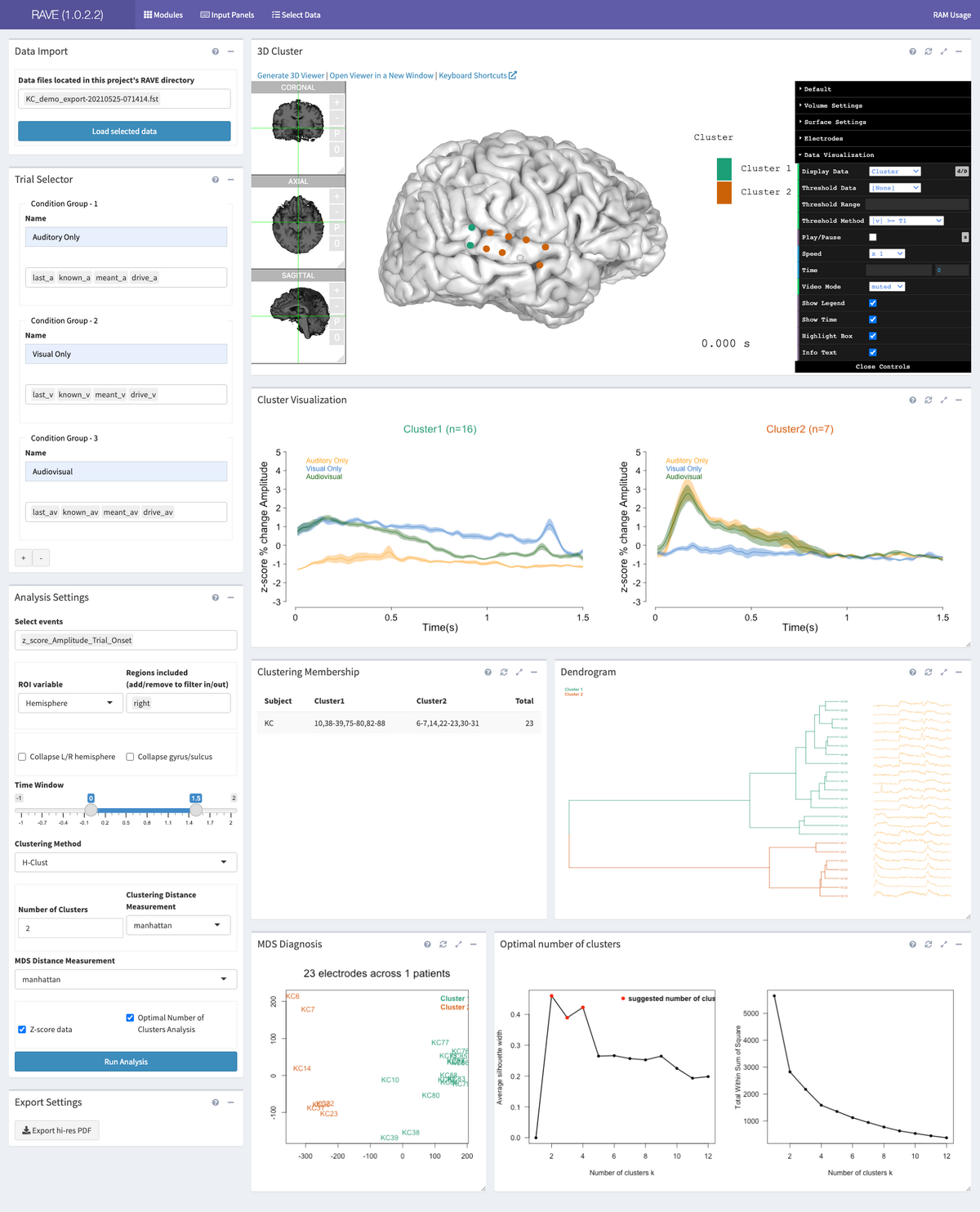
Click the option “Select Data” from the top menu and enter a subject’s referenced data to load. In this tutorial, we would choose "Project: demo" and "Subject: KC". Make sure “Load for Group Analysis” checkbox has been checked. Click “>Load Data” at the bottom right corner of the panel to launch the RAVE session with this subject. Look to the black menu at the left and select “Electrode Clustering.” This page contains multiple panels and plots; this tutorial will use KC_demo as an example to cover them from top to bottom in two columns, as they appear on the page, and from left to right.

Data Import

After loading data, click the multi-selection box on the top left, choose 'KC_demo.fst', then click “>Load Data” to load data.

Trial Selector

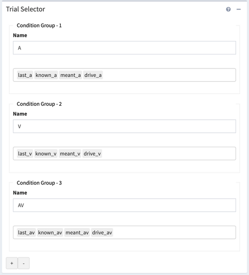
The panel allows us to compare different trial conditions, while the trial condition information has been encoded in the .fst file. In this experiment, we showed participants movie clips of one-syllable words (drive, known, last, meant). The clips were presented either audiovisually (*_av), audio-alone (*_a), or video-alone (*_v).

The conditions would be loaded and automatically grouped as “A: drive_a, known_a, last_a, known_a”, “V: drive_v, known_v, last_v, known_v”, and “AV: drive_av, known_av, last_av, known_av”. These three labels stand for "Auditory only","Visual only", and "Audiovisual" accordingly.

To add a condition group, press the plus icon at the bottom of the panel, and to remove a condition group from analysis, press the minus icon. Under the Name textbox, the droplist of trial conditions selects which trial condition would be included in this condition group.

Analysis Settings

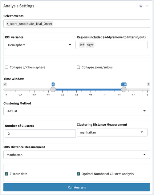
The third panel on the left side of the page is the "Analysis Settings" panel. This panel set the analysis parameters and clustering method for the clustering analysis.

Set the analysis parameters as:

1. Select the events as 'z_score_Amplitude_Trial_Onset'
2. Set ROI variables

Here we select ROI variable as 'Hemisphere', and Region included as 'left'

3. Collapse or not

In this case, we tend to inspect the electrodes from each hemisphere and gyrus/sulcus individually, so we would leave these checkboxes unchecked.

4. Time Window

We would set the start time as 0s, and the end time as 1.5s.

5. Clustering Method

There are two clustering methods available, Hierachical clustering and K-means clustering. We choose Hierachical clustering in this case.

6. Clustering settings

Here we set the number of clusters as 2, clustering distance measurement as 'Manhattan', which is a L-1 distance measurement.

7. Z-score

We prefer to z-score the data before clustering to eliminate the influence of the different amplitude but focus on the shape and trend, thus we check the z-score checkbox.

8. Optimal number of cluster analysis

Here we check the optimal number of cluster analysis to use the silhouette method and elbow method to help decide the optimal cluster number.

After setting all the parameters, click “>Run Analysis” on the bottom to start running the clustering analysis.

Copy plots to PowerPoint

RAVE graphs are quite customizable. Checkout the "Configure plots" input panel and explore some of the options. Some of our favorites include playing with the "Lines color palette", the "Heatmap color palette" or setting "Plot background color " to emulate dark mode. Once you have a plot setup, you can copy it directly into PowerPoint.

nota bene. You can control the width of RAVE plots by resizing your browser window (for even more horizontal space, hide the "Input Panels" by clicking that link in purple bar). The height of plots is controlled by click-and-drag on the bottom-right of the plot. Once resized, you'll need to "refresh" that panel (no recalculation required) by clicking the refresh icon in the upper-right of that output panel.

1. Open Power Point
2. Back in your RAVE browser window, find a graph you like
3. Right-click -> Copy Image
4. Paste the image into your PowerPoint Slide
5. Repeat 2-4 as needed

For capturing the 3dViewer, choose "Open Controls" in the top-right of the "Results on surface" output panel, then "Screenshot".