IGEM:IMPERIAL/2008/Modelling/Tutorial1
<html> <style type="text/css"> .firstHeading {display: none;} </style> </html> <html> <style type="text/css">
table.calendar { margin:0; padding:2px; }
table.calendar td { margin:0; padding:1px; vertical-align:top; } table.month .heading td { padding:1px; background-color:#FFFFFF; text-align:center; font-size:120%; font-weight:bold; } table.month .dow td { text-align:center; font-size:110%; } table.month td.today { background-color:#3366FF } table.month td {
   border:2px;
   margin:0;
   padding:0pt 1.5pt;
   font-size:8pt;
   text-align:right;
   background-color:#FFFFFF;
   }
- bodyContent table.month a { background:none; padding:0 }
.day-active { font-weight:bold; } .day-empty { color:black; } </style> </html>
| <html><a href=http://openwetware.org/wiki/IGEM:IMPERIAL/2008/Prototype><img width=50px src=http://openwetware.org/images/f/f2/Imperial_2008_Logo.png></img</a></html> | Home | The Project | B.subtilis Chassis | Wet Lab | Dry Lab | Notebook |
|---|
<html> <style type="text/css"> div.Section { font:11pt/16pt Calibri, Verdana, Arial, Geneva, sans-serif; }
/* Text (paragraphs) */ div.Section p { font:11pt/16pt Calibri, Verdana, Arial, Geneva, sans-serif; text-align:justify; margin-top:0px; margin-left:30px; margin-right:30px; }
/* Headings */ div.Section h1 { font:22pt Calibri, Verdana, Arial, Geneva, sans-serif; text-align:left; color:#3366FF; }
/* Subheadings */ div.Section h2 { font:18pt Calibri, Verdana, Arial, Geneva, sans-serif; color:#3366FF; margin-left:5px; }
/* Subsubheadings */ div.Section h3 { font:16pt Calibri, Verdana, Arial, sans-serif; font-weight:bold; color:#3366FF; margin-left:10px; }
/* Subsubsubheadings */ div.Section h4 { font:12pt Calibri, Verdana, Arial, sans-serif; color:#3366FF; margin-left:15px; }
/* Subsubsubsubheadings */ div.Section h5 { font:12pt Calibri, Verdana, Arial, sans-serif; color:#3366FF; margin-left:20px; }
/* References */ div.Section h6 { font:12pt Calibri, Verdana, Arial, sans-serif; font-weight:bold; font-style:italic; color:#3366FF; margin-left:25px; }
/* Hyperlinks */ div.Section a {
}
div.Section a:hover {
}
/* Tables */ div.Section td { font:11pt/16pt Calibri, Verdana, Arial, Geneva, sans-serif; text-align:justify; vertical-align:top; padding:2px 4px 2px 4px; }
/* Lists */ div.Section li { font:11pt/16pt Calibri, Verdana, Arial, Geneva, sans-serif; text-align:left; margin-top:0px; margin-left:30px; margin-right:0px; }
/* TOC stuff */ table.toc { margin-left:10px; }
table.toc li { font: 11pt/16pt Calibri, Verdana, Arial, Geneva, sans-serif; text-align: justify; margin-top: 0px; margin-left:2px; margin-right:2px; }
/* [edit] links */ span.editsection { color:#BBBBBB; font-size:10pt; font-weight:normal; font-style:normal; vertical-align:bottom; } span.editsection a { color:#BBBBBB; font-size:10pt; font-weight:normal; font-style:normal; vertical-align:bottom; } span.editsection a:hover { color:#3366FF; font-size:10pt; font-weight:normal; font-style:normal; vertical-align:bottom; }
- sddm {
margin: 0; padding: 0; z-index: 30 }
- sddm li {
margin: 0; padding: 0; list-style: none; float: center; font: bold 12pt Calibri, Verdana, Arial, Geneva, sans-serif; border: 0px }
- sddm li a {
display: block; margin: 0px 0px 0px 0px; padding: 0 0 12px 0; background: #33bbff; color: #FFFFFF; text-align: center; text-decoration: none; }
- sddm li a:hover {
border: 0px }
- sddm div {
position: absolute; visibility: hidden; margin: 0; padding: 0; background: #33bbff; border: 1px solid #33bbff } #sddm div a { position: relative; display: block; margin: 0; padding: 5px 10px; width: auto; white-space: nowrap; text-align: left; text-decoration: none; background: #FFFFFF; color: #2875DE; font: 11pt Calibri, Verdana, Arial, Geneva, sans-serif } #sddm div a:hover { background: #33bbff; color: #FFFFFF } </style></html>
Data
There are 3 types of data:
- Synthetic Data
The OECD defines synthetic data as: "An approach to confidentiality where instead of disseminating real data, synthetic data that have been generated from one or more population models are released." [1]
Simply put, synthetic data is realistic data with well understood characteristics, generated by the user. The process of generating synthetic data may be based on well studied models. Uses of synthetic data include evaluating new research ideas and testing the performance of systems. The user is also able to cover more data space through generation of synthetic data, an advantage over real data which the user does not have control of.
- Phantom Data
Phantom data is data obtained from a phantom model which is a realistic system being generated by the user. This type of data is often found when the real system is difficult to obtain but can be modeled. For example, a human skull phantom can be used to obtain EEG phantom data [2], or a heart phantom can be used to obtain imaging phantom data [3].
- Real Data
Real data, is of course data obtained from a real-life sample set. Real data can be classified into discrete and continuous data. Discrete data can follow a binomial, poisson or a uniform distribution, whereas continuous data follow a uniform distribution, and in most cases, a normal distribution.
In our case we use synthetic data to conduct our pre-experimental analyses and design our experiments.
Model Construction
List the relevant properties of the movement of B. subtilis and turn them into an adequate model (or even better a family of models).
Here is a possible model.
- Running Phase
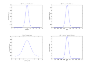
Bacteria move at constant velocity v in direction θ for a period of time t.
- v drawn from Gaussian distribution of mean v0 and standard deviation σ1.
- t drawn from Gaussian distribution of mean t0 and standard deviation σ2.
- Simulations: v0=10μm/s and t0=1s. Take σ1=v0/10 and σ2=t0/10
- Plot the distributions of v and t
- Rotating Phase
Bacteria stop for a period of time T and rotate by an angle α.
- T drawn from Gaussian of mean Tr and standard deviation σr.
- α drawn from Von Mises distribution of mean α0 and parameter β.
- Simulations: α0=0 and T=0.1s. Take β=1 and σs=T/10
- Plot the distributions of α and T
- Useful m-file
Random number generator. This generates distributions including the normal and von Mises distributions. Save as randraw.m in the same folder as your model.
 %Model Construction of Bacteria Motility


 %Gaussian distribution of velocity
 v=[1:0.01:20];                %Range of velocities
 v_avg=10;                     %Average velocity v0
 v_dev=v_avg/10;               %Standard Deviation sigma-1
 y1=normpdf(v,v_avg,v_dev);    %Generation of PDF of velocities
 subplot(2,2,1);
 plot(v,y1);
 title('PDF of Bacteria "Run" Velocity')
 xlabel('Velocity'); ylabel('Probability Density');


 %Gaussian distribution of run-time
 t=[0:0.001:2];                %Range of run duration
 t_avg=1;                      %Average run duration
 t_dev=t_avg/10;               %Standard Deviation sigma-2
 y2=normpdf(t,t_avg,t_dev);    %Generation of PDF of run duration
 subplot(2,2,2); plot(t,y2);
 title('PDF of Bacteria "Run" Duration')
 xlabel('Time'); ylabel('Probability Density');


 % Distribution of angles
 x=[-pi:0.01:pi];              %Range of angle theta
 x_avg=0;                      %Average turn angle
 k=1;                          %Beta factor
 b=besselj(0,k); %Generates a Bessel function of first kind and order 0
 y3=(1/(2*pi*b))*exp(k*cos(x-x_avg)); %Generates the Von Mises distribution
 subplot(2,2,3);
 plot(x,y3);
 Title('PDF of Tumbling Angle');
 xlabel('Tumbling Angle'); ylabel('Probability Density');


 % Distribution of tumbling-time
 ts=[0:0.001:0.2];             %Range of tumbling duration
 ts_avg=0.1;                   %Average tumbling duration
 ts_dev=ts_avg/10;             %Standard Deviation sigma-s
 y4=normpdf(ts,ts_avg,ts_dev); %Gernation of PDF of tumbling duration
 subplot(2,2,4); plot(ts,y4);
 title('PDF of Bacteria "Tumbling" Duration')
 xlabel('Time'); ylabel('Probability Density');
Simulations

We suppose that we will be able to shoot short movies of a few bacteria moving in a medium of our choice. This is dependent on development and implementation of protocols to successfully culture our bacteria, and suitable training and expertise on the microscope! With the use of appropriate software the position of a few bacteria can be tracked with time. This will give us data in the form of position co-ordinates with tiem.
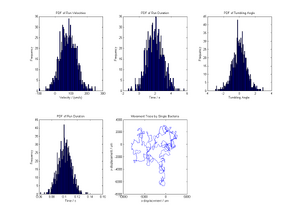
Generation of Realistic Synthetic Data Using the previously constructed model:
- Simulate the run of a handful of bacteria over 5 minutes.
- If possible create a little movie (for the Jamboree presentation.
- Store these data – they will be precious for the data analysis phase that will be developed in the next tutorial.
 clear all;

 %Generation of bacteria run data
 theta=zeros(300,1);                   %Declares 300x1 matrice for turn angle
 theta=randraw('vonmises',[0,1],300);  %Generates tumbling angle

 x=zeros(300,1);
 y=zeros(300,1);

 for n=1:300
     plot(x,y,'b.-');
     v_run(n)=normrnd(10,1);            %Generates run speed
     t_run(n)=normrnd(1,0.1);           %Generates run duration
     t_tumb(n)=normrnd(0.1,0.01);       %Generates tumbling duration
     M(n)=getframe;
     if n==1;
         beta(n)=0;                     %Initialise cummulative angle to 0
         x(n)=0;                        %Initialise origin to (x,y)=(0,0)
         y(n)=0;
     else
         beta(n)=beta(n-1)+theta(n-1);  %Generates cummulative turn angle
         x(n)=x(n-1)+v_run(n)*cos(beta(n))*t_run(n);    %Displacement=Velocity*Time
         y(n)=y(n-1)+v_run(n)*sin(beta(n))*t_run(n);
     end;
 end;

 movie2avi(M,'Motility.avi');

 figure
 subplot(2,3,1); hist(v_run,300);  %Plots histogram of run velocity
 Title('PDF of Run Velocities');
 xlabel('Velocity / (um/s)'); ylabel('Frequency');

 subplot(2,3,2); hist(t_run,300);  %Plots histogram of run duration
 Title('PDF of Run Duration');
 xlabel('Time / s'); ylabel('Frequency');

 subplot(2,3,3); hist(theta,300);  %Plots histogram of turn angle
 Title('PDF of Tumbling Angle');
 xlabel('Tumbling Angle'); ylabel('Frequency');

 subplot(2,3,4); hist(t_tumb,300); %Plots histogram of tumbling duration
 Title('PDF of Run Duration');
 xlabel('Time / s'); ylabel('Frequency');

 subplot(2,3,5); plot(x,y);        %Plots 2D displacement
 Title('Movement Trace by Single Bacteria');
 xlabel('x-displacement / um');
 ylabel('y-displacement / um');

 %Calculate statistical data from synthetic data generated

 v_run_mu=mean(v_run)      %Calculate mean run velocity
 t_run_mu=mean(t_run)      %Calculate mean run duration
 t_tumb_mu=mean(t_tumb)    %Calculate mean tumbling time
 theta_mu=mean(theta)      %Calculate mean turn angle

 v_run_sigma=std(v_run)    %Calculate run velocity standard deviation
 t_run_sigma=std(t_run)    %Calculate run duration standard deviation
 t_tumb_sigma=std(t_tumb)  %Calculate tumbling duration standard deviation
 theta_sigma=std(theta)    %Calculate turn angle standard deviation
Generation of Unrealistic Synthetic Data
Build another model with a running phase and a rotating phase. This time, deliberately make the velocity, time and angle distributions unrealistic.
The unrealistic data set assumes uniform distributions for the velocity, time and angle of rotation.
- Simulate the run of a handful of bacteria over 5 minutes.
- Create a little movie (for the Jamboree presentation)
- Store these data – they will also be precious for the data analysis phase that will be developed in the next tutorial.
v_avg = input('What is the mean velocity of the bacteria?');
t_avg = input('What is the mean run time?');
time = input('How many measurements?');

v_run=(2*v_avg)*(rand(time,1));          %uniformly distributed run velocities
t_run=(2*t_avg)*(rand(time,1));          %uniformly distributed run durations
theta=(2*pi)*(rand(time,1))-pi;       %tumbling angles

beta=zeros(time,1);  %for storage of beta
x=zeros(time,1);     %for storage of x
y=zeros(time,1);     %for storage of y

for n=2:time

beta(n)=beta(n-1)+theta(n-1);  %Generates cummulative turn angle
x(n)=x(n-1)+v_run(n)*cos(beta(n))*t_run(n);    %Displacement=Velocity*Time
y(n)=y(n-1)+v_run(n)*sin(beta(n))*t_run(n);

end

results = [beta,x,y];

movie2avi(M,'Motility.avi');

%Calculate statistical data from synthetic data generated

v_run_mu=mean(v_run)      %Calculate mean run velocity
t_run_mu=mean(t_run)      %Calculate mean run duration
theta_mu=mean(theta)      %Calculate mean turn angle

v_run_sigma=std(v_run)    %Calculate run velocity standard deviation
t_run_sigma=std(t_run)    %Calculate run duration standard deviation
theta_sigma=std(theta)    %Calculate turn angle standard deviation

subplot(2,2,1); hist(v_run,time);  %Plots histogram of run velocity
Title('PDF of Run Velocities');
xlabel('Velocity / (um/s)'); ylabel('Frequency');

subplot(2,2,2); hist(t_run,time);  %Plots histogram of run duration
Title('PDF of Run Duration');
xlabel('Time / s'); ylabel('Frequency');

subplot(2,2,3); hist(theta,time);  %Plots histogram of turn angle
Title('PDF of Tumbling Angle');
xlabel('Tumbling Angle'); ylabel('Frequency');

subplot(2,2,4); plot(x,y);        %Plots 2D displacement
Title('Movement Trace by Single Bacteria');
xlabel('x-displacement / um');
ylabel('y-displacement / um');
Qualitative Description of the motion of bacteria
Arguably one of the greatest challenges of Synthetic Biology is the transitions from qualitative to quantitative summaries of experimental results. An example of a qualitative description would be the characterisation of a biobrick via a spec sheet. In general a simple biological process can be described quantitatively. Whether a complex process, or the interactions between many processes, can also be quantified or described mathematically is an open question.
It is informative to consider the advantages of a quantitative description. To do this, Let us try to find out when a qualitative description is enough and when it needs complementing. Synthetic data are ideal to conduct this kind of study since we control everything in the study and know the underlying truth.
Qualitative descriptions of the above models are given.
However, the traces produced using each data set are indistiguishable when plotted as (x,y) coordinates in time. Thus it is informative to have the (concise) quantitative description of the model as well as a plot.
In the second and third tutorials we will see that obtaining a quantitative description is not that easy and often a certain amount of uncertainty remains at the end of the analysis.
References
-
Definition of Synthetic Data [1]
- Leahy RM, Mosher JC, Spencer ME, Huang MX, and Lewine JD. A study of dipole localization accuracy for MEG and EEG using a human skull phantom. Electroencephalogr Clin Neurophysiol. 1998 Aug;107(2):159-73. DOI:10.1016/s0013-4694(98)00057-1 |
-
Normal and Pathological NCAT Image and Phantom Data Based on Physiologically Realistic Left Ventricle Finite-Element Models Alexander I. Veress, W. Paul Segars, Member, IEEE, Jeffrey A. Weiss, Benjamin M. W. Tsui, Fellow, IEEE, and Grant T. Gullberg, Fellow, IEEE[1]
<html>
|
|
|