IGEM:IMPERIAL/2006/project/Oscillator/Theoretical Analyses/3Dto2D
From OpenWetWare
Jump to navigationJump to search
Analysis of the Model of the Molecular Predation Oscillator
Model Simplification
- Why we can simplify the 3d Model into a 2D Model
- Simplification is possible because of the similarity of the growth rates of the predator terms (V and W) in the 3D Model
- Their complex production terms are identical
- Only their dissipative terms (-d1*V and -d2*W ) varies
- A simple hypotheses could lead to a very big simplification in our analysis
- A 2D analysis is much simpler, and still will give us valid prediction on whether the system will oscillate.
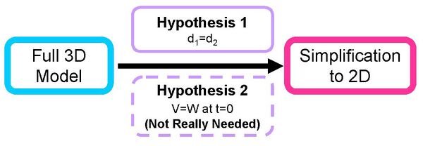
- Required Hypotheses for Simplification
- Hypothesis 1: to ensure V and W have same growth rates
- Hypothesis 1: d1=d2)
- Hypothesis 2:To have equality of the initial conditions
- Hypothesis 2: [aiiA] = [LuxR] at time t=0
- Under previous 2 Hypotheses
- aiiA and LuxR start at the same concentration
- they have the same rate of production and degradation
- hence they have at the same concentration throughout
- System then can be simplified to


- Validity of the hypotheses
- Hypothesis 1 : d1=d2
- The assumption of d1=d2 is feasible because aiiA and LuxR within the cells will be washed out at the same rate in chemostat.
- As long as we can ensure the washing out rate is much more dominant than their natural half-life (easily achieved) the assumption should hold
- Hypothesis 2 is not really essential
- it is fortunate as it was hard to ensure
- if d1=d2, the difference between W and V will decay to 0 exponentially (with a time constant 1/d1)
- therefore after a little time we can assume V=W
- the larger d1, the faster the assumption becomes valid
- the larger the difference between initial values of V & W, the longer the settling time of reaching V=W only
- In particular we are sure that the condition on the parameters for obtaining a limit cycle will still be identical in 2D and 3D despite of the initial concentrations of U V W.
- Problem : in Theory , there is a Huge Difference Between 2D and 3D
- Poincare-Bendixson Theorem works for 1D and 2D only, but not 3D
- We only need simple requirements for a limit cycle in 2D
- In 3D the requirement is more complex - or much more complex
- So are our results in 2D worth anything ?
- If our hypotheses are exactly met: Yes!
- In practice hypotheses not exactly met, but we have a margin of error
- A slight error on Hypothesis 2 is not important
- Slight error on hypothesis 1 (d1 not strictly equal to d2): 2 Scenarii
- Scenario 1: (the kind one)
- For d1=d2 and a range of parameters well chosen we have oscillations
- Because the system is well behaved , we still have oscillations at the vicinity of these parameters (hence for d1 slightly different from d2)
- Scenario 2: (the not so nice one)
- [aiiA] and [LuxR] get more and more out of synchronisation
- However, if the hypotheses are almost met, we can hope to have a few synchronised cycles
- Conclusion
- There is a lot to learn from the 2D model
- A word of caution:
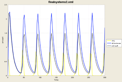
- The simulation above shows individual cycles of [aiiA] and [LuxR]
- Frequencies are equal
- Profiles very similar
- Peak amplitudes different
- Clearly for such cycles d1=d2 was not met and yet we have oscillations. We therefore have to study the 3D case in its entirety at some point
- However for our current interest of whether the system can result in generation, 2D case of d1=d2 should be enough
- The simulation above shows individual cycles of [aiiA] and [LuxR]
<html>
<script type="text/javascript" language="javascript">
var sc_project=1999441;
var sc_invisible=1;
var sc_partition=18;
var sc_security="18996820";
</script>
<script type="text/javascript" language="javascript" src="http://www.statcounter.com/counter/frames.js"></script><noscript><a href="http://www.statcounter.com/" target="_blank"><img src="http://c19.statcounter.com/counter.php?sc_project=1999441&java=0&security=18996820&invisible=1" alt="website statistics" border="0"></a> </noscript> </html>
