User:Justin Roth Muehlmeyer/Notebook/307L Notebook/Poisson
Set Up
Searching for the cosmic radiation signals:
Using a Tektronix 485 Oscilloscope (analog) and ORTEC model # 266 PM base.
Dynode output on PMT to oscilloscope Input Voltage -1500 V PMT outside of lead brick cave
Analog Oscilloscope settings:
- 5 mV/division
- 1 ms/division
- AC triggering: negative slope (internal)
We observe occasional peaks per second that are distinguishable from noise. They change so fast that we cant actually measure the amplitude of their peaks. This is our presumed cosmic radiation.
Using an amplifier:
- We addded a ORTEC amplifier to our board, and connected the output of the diode to the input of the amplifyer. We wanted to test the signal coming out of the amplifier with the oscilloscope before connecting it into the computer. We ran into many difficulties even finding our cosmic radiation signal with the amplifier, and then again while bypassing it.
We had extensive difficulties in trying to get a signal of the cosmic radiation using the amplifier.
Troubleshooting:
New amplifier: Canberra PAD 814.
Switched from dynode to the anode on the PMT, with no effect.
Switched to new PMT - Tracor Northern Model # TN1222. Way clearer, greater magnitude cosmic radiation spikes with just the oscilloscope. Input ~-1400 V. Positive V output.
Still no results from the amplifier, so...
New Oscilloscope: Tektronix TDS 1002 (digital).
"Derivative signal" from the amplifier. Set up: PMT to PREAMP IN, PREAMP switch to IN, AMP OUT to oscilloscope (DC coupling, rising slope, 36.0 mV)
Hooking it up to the software (MCA):
Software: PCA3 in MSDOS Bins: 512 We decided to first take our dwell time to be 1 second.
Other passes: dwell time of 1, 100, 10000 microseconds,
Data
The data we received in the computer was outputed to ASCII file type, which I will post here. The following was the data taken for the 1s trial.
Sep 22 2008 4:01:29 pm Elt: 000000 Seconds. Real Time: 000000 ID: No spectrum identifier defined Memory Size: 16384 Chls Conversion Gain: 0256 Adc Offset: 0000 Chls
Chn    Counts  ROI
  0,       16, 000
  1,       16, 000
  2,       12, 000
  3,       12, 000
  4,       13, 000
  5,       12, 000
  6,       14, 000
  7,       11, 000
  8,       12, 000
  9,       11, 000
 10,       13, 000
 11,       14, 000
 12,       15, 000
 13,       14, 000
 14,       13, 000
 15,       14, 000
 16,       17, 000
 17,       14, 000
 18,       14, 000
 19,       14, 000
 20,       14, 000
 21,       14, 000
 22,       14, 000
 23,       11, 000
 24,       16, 000
 25,       13, 000
 26,       10, 000
 27,       15, 000
 28,       17, 000
 29,       11, 000
 30,       13, 000
 31,       11, 000
 32,       12, 000
 33,       14, 000
 34,       14, 000
 35,       13, 000
 36,       11, 000
 37,       12, 000
 38,       13, 000
 39,       13, 000
 40,       16, 000
 41,       13, 000
 42,       14, 000
 43,       11, 000
 44,       15, 000
 45,       16, 000
 46,       13, 000
 47,       11, 000
 48,       12, 000
 49,       11, 000
 50,       16, 000
 51,       13, 000
 52,       15, 000
 53,       15, 000
 54,       10, 000
 55,       17, 000
 56,       14, 000
 57,       17, 000
 58,       16, 000
 59,       13, 000
 60,       14, 000
 61,       16, 000
 62,       13, 000
 63,       11, 000
 64,       13, 000
 65,       16, 000
 66,       10, 000
 67,       16, 000
 68,       12, 000
 69,       17, 000
 70,       13, 000
 71,       11, 000
 72,       13, 000
 73,       16, 000
 74,       13, 000
 75,       14, 000
 76,       12, 000
 77,       14, 000
 78,       14, 000
 79,       13, 000
 80,       12, 000
 81,       11, 000
 82,       15, 000
 83,       15, 000
 84,       13, 000
 85,       14, 000
 86,       10, 000
 87,       14, 000
 88,       15, 000
 89,       20, 000
 90,       13, 000
 91,       14, 000
 92,       10, 000
 93,       14, 000
 94,       13, 000
 95,       12, 000
 96,       12, 000
 97,       14, 000
 98,       15, 000
 99,       14, 000
100,       14, 000
101,       13, 000
102,       13, 000
103,       11, 000
104,       16, 000
105,       14, 000
106,        9, 000
107,       18, 000
108,        9, 000
109,       15, 000
110,       11, 000
111,       16, 000
112,       14, 000
113,       12, 000
114,       15, 000
115,       16, 000
116,       16, 000
117,       13, 000
118,       14, 000
119,       16, 000
120,       16, 000
121,       13, 000
122,       15, 000
123,       15, 000
124,       12, 000
125,       16, 000
126,       11, 000
127,       13, 000
128,       14, 000
129,       15, 000
130,       15, 000
131,       10, 000
132,       12, 000
133,       13, 000
134,       15, 000
135,       12, 000
136,       16, 000
137,       14, 000
138,       12, 000
139,       15, 000
140,       19, 000
141,       13, 000
142,       15, 000
143,       11, 000
144,       16, 000
145,       16, 000
146,       13, 000
147,       13, 000
148,       13, 000
149,       15, 000
150,       14, 000
151,       13, 000
152,       14, 000
153,       12, 000
154,       14, 000
155,       15, 000
156,       15, 000
157,       14, 000
158,       13, 000
159,       16, 000
160,       12, 000
161,       15, 000
162,       14, 000
163,       11, 000
164,       15, 000
165,        8, 000
166,       10, 000
167,       15, 000
168,       17, 000
169,       11, 000
170,       15, 000
171,       11, 000
172,       12, 000
173,       15, 000
174,       18, 000
175,       12, 000
176,       11, 000
177,       11, 000
178,       10, 000
179,       15, 000
180,       14, 000
181,       12, 000
182,       17, 000
183,       10, 000
184,       18, 000
185,       13, 000
186,       15, 000
187,       14, 000
188,       14, 000
189,       15, 000
190,       12, 000
191,       17, 000
192,       10, 000
193,       11, 000
194,       14, 000
195,       14, 000
196,       11, 000
197,       15, 000
198,       14, 000
199,       13, 000
200,       13, 000
201,       18, 000
202,       10, 000
203,       14, 000
204,       12, 000
205,       11, 000
206,       16, 000
207,       11, 000
208,       11, 000
209,       13, 000
210,       16, 000
211,       12, 000
212,       15, 000
213,       16, 000
214,       12, 000
215,       14, 000
216,       17, 000
217,       14, 000
218,       12, 000
219,       16, 000
220,       15, 000
221,       17, 000
222,       14, 000
223,       16, 000
224,       18, 000
225,       15, 000
226,       15, 000
227,       12, 000
228,       11, 000
229,       13, 000
230,       14, 000
231,       15, 000
232,       14, 000
233,       15, 000
234,       13, 000
235,       17, 000
236,       14, 000
237,       12, 000
238,       13, 000
239,       12, 000
240,        8, 000
241,       13, 000
242,       14, 000
243,        9, 000
244,       14, 000
245,       18, 000
246,       14, 000
247,       12, 000
248,       16, 000
249,       14, 000
250,       15, 000
251,       13, 000
252,       14, 000
253,       14, 000
254,       13, 000
255,       16, 000
256,       14, 000
257,       17, 000
258,       16, 000
259,       13, 000
260,       14, 000
261,        9, 000
262,       15, 000
263,       14, 000
264,       16, 000
265,       13, 000
266,       15, 000
267,       14, 000
268,       12, 000
269,       13, 000
270,       14, 000
271,       13, 000
272,       15, 000
273,       12, 000
274,       14, 000
275,       13, 000
276,       13, 000
277,       13, 000
278,       10, 000
279,       15, 000
280,       16, 000
281,       13, 000
282,       16, 000
283,       13, 000
284,       14, 000
285,       10, 000
286,       13, 000
287,       15, 000
288,       14, 000
289,       13, 000
290,       17, 000
291,       15, 000
292,       11, 000
293,       11, 000
294,       16, 000
295,       14, 000
296,       14, 000
297,       16, 000
298,        9, 000
299,       12, 000
300,       12, 000
301,       15, 000
302,       13, 000
303,       10, 000
304,       14, 000
305,       15, 000
306,       12, 000
307,       11, 000
308,       12, 000
309,       13, 000
310,       16, 000
311,       12, 000
312,        8, 000
313,       15, 000
314,       14, 000
315,       16, 000
316,       10, 000
317,       13, 000
318,       13, 000
319,       12, 000
320,       13, 000
321,       12, 000
322,       17, 000
323,       14, 000
324,       14, 000
325,       14, 000
326,       12, 000
327,       14, 000
328,       16, 000
329,       14, 000
330,       10, 000
331,       14, 000
332,       14, 000
333,       14, 000
334,       14, 000
335,       12, 000
336,       16, 000
337,       13, 000
338,       10, 000
339,       12, 000
340,       12, 000
341,       11, 000
342,       15, 000
343,       16, 000
344,       10, 000
345,       13, 000
346,       13, 000
347,       13, 000
348,       10, 000
349,       14, 000
350,       15, 000
351,       14, 000
352,       13, 000
353,       14, 000
354,       16, 000
355,       14, 000
356,       18, 000
357,        9, 000
358,       13, 000
359,       14, 000
360,       10, 000
361,       11, 000
362,       13, 000
363,       15, 000
364,       15, 000
365,       14, 000
366,       11, 000
367,       17, 000
368,       13, 000
369,       11, 000
370,       15, 000
371,       16, 000
372,       16, 000
373,       13, 000
374,       13, 000
375,       13, 000
376,       11, 000
377,       15, 000
378,       10, 000
379,       11, 000
380,       16, 000
381,       15, 000
382,       16, 000
383,       14, 000
384,       18, 000
385,       13, 000
386,       14, 000
387,       16, 000
388,       14, 000
389,       14, 000
390,       12, 000
391,       12, 000
392,       13, 000
393,        8, 000
394,       18, 000
395,       14, 000
396,        7, 000
397,       13, 000
398,       11, 000
399,       13, 000
400,       11, 000
401,       15, 000
402,       12, 000
403,       14, 000
404,       10, 000
405,       12, 000
406,       16, 000
407,       15, 000
408,       13, 000
409,       14, 000
410,       12, 000
411,       11, 000
412,       13, 000
413,       13, 000
414,       17, 000
415,       13, 000
416,       13, 000
417,       15, 000
418,       13, 000
419,       16, 000
420,       14, 000
421,       12, 000
422,        9, 000
423,       16, 000
424,       12, 000
425,       13, 000
426,       15, 000
427,       14, 000
428,       12, 000
429,       11, 000
430,       16, 000
431,       11, 000
432,       14, 000
433,       16, 000
434,        7, 000
435,       15, 000
436,       15, 000
437,       13, 000
438,       14, 000
439,       12, 000
440,       11, 000
441,       12, 000
442,       13, 000
443,       15, 000
444,       12, 000
445,       15, 000
446,       13, 000
447,       14, 000
448,       13, 000
449,       15, 000
450,       12, 000
451,       11, 000
452,       16, 000
453,       16, 000
454,       15, 000
455,       14, 000
456,       12, 000
457,       12, 000
458,       13, 000
459,       13, 000
460,       12, 000
461,       14, 000
462,       15, 000
463,       13, 000
464,       13, 000
465,       16, 000
466,       14, 000
467,       13, 000
468,       14, 000
469,       15, 000
470,       17, 000
471,       14, 000
472,       13, 000
473,        8, 000
474,       12, 000
475,       15, 000
476,       16, 000
477,       11, 000
478,       13, 000
479,       12, 000
480,       14, 000
481,       13, 000
482,       13, 000
483,       15, 000
484,       14, 000
485,       14, 000
486,       11, 000
487,       14, 000
488,       12, 000
489,       13, 000
490,       14, 000
491,       12, 000
492,       15, 000
493,       11, 000
494,        8, 000
495,       18, 000
496,       14, 000
497,       14, 000
498,       12, 000
499,       11, 000
500,       12, 000
501,       15, 000
502,       10, 000
503,       12, 000
504,       14, 000
505,       16, 000
506,       14, 000
507,       16, 000
508,       14, 000
509,       12, 000
510,       13, 000
511,       15, 000
Results
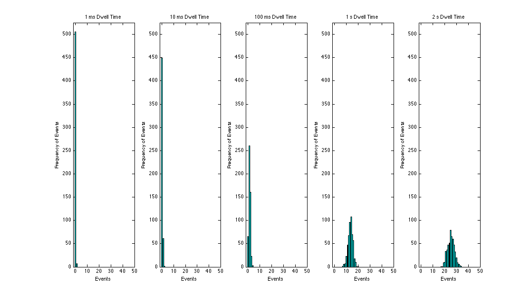
Using Mr. Barron's amazing Matlab skills our results were as follows for each dwell time:
Here is the code for this:
%% Poisson Distribution Analysis

% Alexander Barron
% Junior Lab Fall 2008

close all, clear all;

%% Load .txt files

M1ms_bin = dlmread('JAND1MS.txt',',',[0 0 511 0]);  % bin vector 1ms dwell
M1ms_val = dlmread('JAND1MS.txt',',',[0 1 511 1]);  % value vector 1ms dwell

M10ms_bin = dlmread('JAND10MS.txt',',',[0 0 511 0]);
M10ms_val = dlmread('JAND10MS.txt',',',[0 1 511 1]);

M100ms_bin = dlmread('JAND100M.txt',',',[0 0 511 0]);
M100ms_val = dlmread('JAND100M.txt',',',[0 1 511 1]);

M1s_bin = dlmread('JAND1S.txt',',',[0 0 511 0]);
M1s_val = dlmread('JAND1S.txt',',',[0 1 511 1]);

M2s_bin = dlmread('JAND2S.txt',',',[0 0 511 0]);
M2s_val = dlmread('JAND2S.txt',',',[0 1 511 1]);


%% sort into frequencies for histograms

d1ms_count = zeros(1,50);       % Here I am creating empty
d10ms_count = zeros(1,50);      % vectors in which to put
d100ms_count = zeros(1,50);     % my manipulated data.
d1s_count = zeros(1,50);
d2s_count = zeros(1,50);

for c=1:5;

    switch c;
        case 1;
            valmat = M1ms_val;          % generic value and
            countmat = d1ms_count;      % count matrices
        case 2;
            valmat = M10ms_val;
            countmat = d10ms_count;
        case 3;
            valmat = M100ms_val;
            countmat = d100ms_count;
        case 4;
            valmat = M1s_val;
            countmat = d1s_count;
        case 5;
            valmat = M2s_val;
            countmat = d2s_count;
    end;

    for j=1:512;                        % Here I scan my data for
                                        % desired frequencies
        for k=0:50;                     % and place them in
                                        % generic matrices.
            if valmat(j) == k;
                countmat(k+1) = countmat(k+1) + 1;
            end

        end

    end

    switch c;
        case 1;
            d1ms_count = countmat;      % transformation of
        case 2;                         % generic matrices
            d10ms_count = countmat;     % into appropriately-
        case 3;                         % named ones
            d100ms_count = countmat;
        case 4;
            d1s_count = countmat;
        case 5;
            d2s_count = countmat;
    end;

    clear valmat, clear countmat;

end;


%% Plot

freq = linspace(0,49,50);

scrsz = get(0,'ScreenSize');
figure('Position',[1 scrsz(4)/1.5 scrsz(3)/1.25 scrsz(4)/1.4]);

for f=1:5;

    switch f;
        case 1;
            data = d1ms_count;
            titl = '1 ms Dwell Time';
        case 2;
            data = d10ms_count;
            titl = '10 ms Dwell Time';
        case 3;
            data = d100ms_count;
            titl = '100 ms Dwell Time';
        case 4;
            data = d1s_count;
            titl = '1 s Dwell Time';
        case 5;
            data = d2s_count;
            titl = '2 s Dwell Time';
    end;

    subplot(1,5,f), bar(freq,data,'c');
    ylim([0 525]);
    xlim([-2 50]);
    set(gca,'XTick',[0 10 20 30 40 50]);
    ylabel('Frequency of Events');
    xlabel('Events');
    title(titl);

    clear data;

end;
Analysis
The Poisson distribution:
- [math]\displaystyle{ f(k; \lambda)=\frac{\lambda^k e^{-\lambda}}{k!},\,\! }[/math]
Calculating the mean:
In the Poisson distribution, the mean and the variance are the same thing, which is λ. λ is the expected rate of events, the expected number of occurences per time interval. To calculate λ I will use the data average method. I sum up the number of events that occurred, and divide by the number of times I took those events.
- [math]\displaystyle{ \widehat{\lambda}_\mathrm{MLE}=\frac{1}{n}\sum_{i=1}^n k_i. \! }[/math]
My excel file data sheet that I used to do this analysis I will place here:
File:Poisson Analysis for lamda Muehlmeyer.xls
The following is a summary of my λ values for each dwell time using the data average method.
- 1ms, λ = 0.013671875
- 10ms, λ = 0.126953125
- 100ms, λ = 1.294921875
- 1s, λ = 13.48828125
- 2s, λ = 25.36132813
This makes sense, as our dwell time increases, our average rate of events increases. And when you compare each of these values to our plots, they are quite apparently the mean.
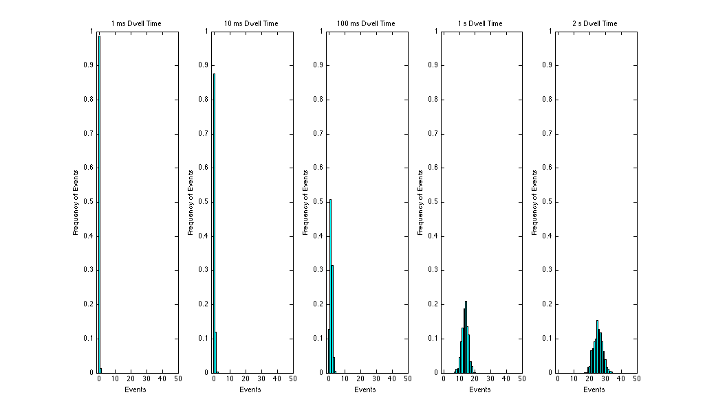
In order to see our results more clearly, we can normalize our results so that they fit a probablity density function that sums to 1. This plots our results as a matter of probabilty. We do this by dividing the frequency of events by the maximimum possibility 512. See the plots below.
What is most interesting is that as we increase the dwell time the histogram plot begins to look like a Gaussian function. The Guassian function peaks at some median value that represents the most common rate of occurences. If we allow for more events (higher dwell time) the histogram then is a plot of this Guassian funtion, which tells us their is a rate of events that occurs the most, and that rate is that at which the Guassian peak appears, our mean, λ.
Error Analysis for λ
SJK 10:34, 20 October 2008 (EDT)

See my comments about this in Der's book
Our error is determined by the deviation from the mean. We found an expression for this value in a formal report from a student from last year. You can see it here at Tomas Mondragon's notebook entry.
[math]\displaystyle{ Error=\frac{\sqrt{\sum_{k=\operatorname{min}\ k}^{\operatorname{max}\ k}\left(f(k,\lambda)-\frac{x_k}{N} \right)^2}}{\sqrt{N}\sqrt{N-1}} }[/math]
Where the frequency count of an event count [math]\displaystyle{ k }[/math] is [math]\displaystyle{ x_k }[/math]. N is 512 in this case.
- 1ms, λ = 0.013671875, λerror = 4.05974132 x 10^-7
- 10ms, λ = 0.126953125, λerror= 1.7313458323 x 10^-5
- 100ms, λ = 1.294921875, λerror= 4.62059546375 x 10^-4
- 1s, λ = 13.48828125, λerror= 3.25904896073 x 10^-4
- 2s, λ = 25.36132813, λerror= 2.4259613547 x 10^-4
Fitting our Data to the Poisson Distribution
The Poisson distribution is characterized by the fact that the standard deviation is equal to the square root of the mean λ. If we can show that this is the case for our data (or atleast reasonably close), then we have shown that our data is in fact a manifestation of the Poisson distribution.
First I will find the standard deviation by assuming that our data is in fact a Poisson distribution (I will take the square root of our calculated λ values):
The number of observed occurences fluctuates about its mean λ with a standard deviation of σk = [math]\displaystyle{ \sqrt{\lambda} }[/math].
- 1ms, λ = 0.013671875, σk = 0.11692
- 10ms, λ = 0.126953125, σk = 0.35650
- 100ms, λ = 1.294921875, σk = 1.13795
- 1s, λ = 13.48828125, σk = 3.67264
- 2s, λ = 25.36132813, σk = 5.03600
This can be roughly validated if one looks at the plots to notice how the distribution deviates out from the mean λ by ±σk.
Now I will determine the standard deviation from our data directly to show that these values for the standard deviation and the values σk above are reasonably close.
This calculation is described by the following formula:
- [math]\displaystyle{ \sigma = \sqrt{\frac{1}{N-1} \sum_{i=1}^N (x_i - \overline{x})^2}\,, }[/math]
Using the excel function for standard deviation (posted above) the standard deviation of our actual data was determined as follows.SJK 10:35, 20 October 2008 (EDT)
This does look correct. However, I don't see the calculations in your actual Excel spreadsheet...just the mean in there.
- 1ms, λ = 0.013671875, σx = 0.116238308
- 10ms, λ = 0.126953125, σx = 0.344790832
- 100ms, λ = 1.294921875, σx = 0.766810045
- 1s, λ = 13.48828125, σx = 2.066378743
- 2s, λ = 25.36132813, σx = 2.945079248
How close are σk and σx?
For low dwell times σx is very close to σk, but as we increase our dwell time the two values begin to differ a bit more. However, I think it is still safe to say that the two values are reasonably close enough to be considered a Poisson distribution.
Why do the two values of σ differ for higher dwell times? Since σ is a measure of deviation of the values from their mean (dispersion), I think that this could be explained by the simple fact that outlyers occur more frequently with longer dwell times, which throw off our data from the ideal Poisson distribution.
Conclusion
The data collection of "random" cosmic radiation events proved to fit the Poisson distribution reasonably well. We also saw how, as we increase the dwell time, this distribution begins to fit a Gaussian with an obvious average rate. We showed our selves that our data is characterized by the fact that the standard deviation is reasonably equal to the square root of the mean λ, which is a charactersistic of the Poisson distribution.
