Practical Finance and Data Analysis Lab Summary
Here is the lab manual page.
Here are my lab notes.
Partner: Justin Muehlmeyer
Introduction
This lab was basically undefined to start with, with simple goals of gathering knowledge on finance in general, learning where to find data, and using data analysis methods to glean information from the data. We came up with several grand ideas, but finally condensed our goals- the entire process can be seen in the lab notes.
Approach
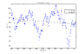
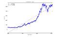
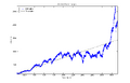
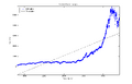
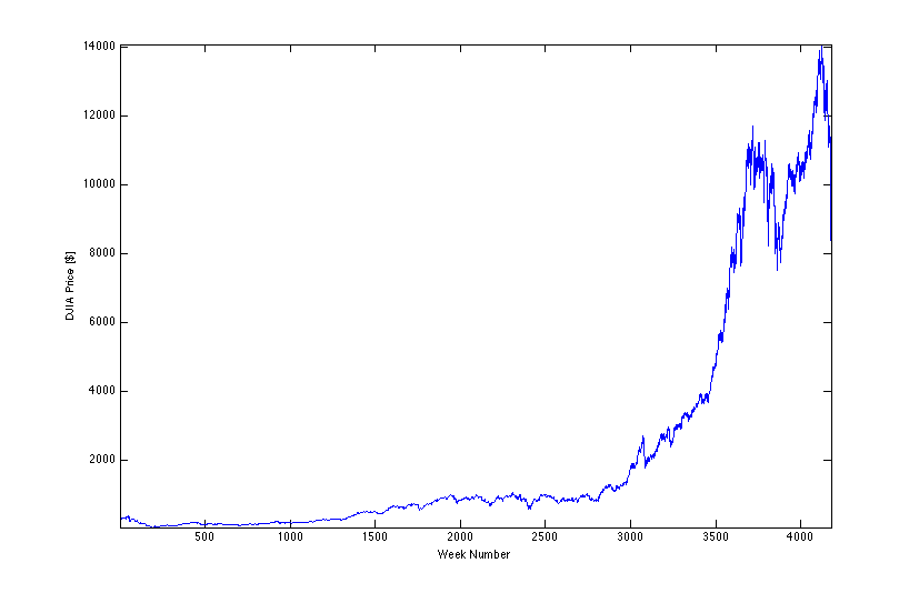
In the end, we generated fixed-length time windows with random start dates over the period of price data acquired for the Dow Jones Industrial Average, then tried to find an average growth rate using both "snapshots" and least-squares linear fits. We defined snapshots as slopes between the start and end points in each time window, reflecting what a person would receive if he actually invested over exactly each window. Least-squares fits take into account fluctuations in the price between the start and end points, so that someone investing on a shorter interval would probably see results more akin to the least-squares fit of his specific time window. We compared the two methods over several different time windows, then analyzed the least-squares data to see if it fit any sort of distribution.
Final Results
Least-squares:
| Least-squares Slope Data [$/week] ± σravg
|
Sample Window
|
| 10 Year Window
|
| 1) 2.4689 ± 0.0007
|
11) 2.6043 ± 0.0007
|
| 2) 3.1063 ± 0.0011
|
12) 3.2287 ± 0.0011
|
| 3) 2.5977 ± 0.0008
|
13) 2.1363 ± 0.0009
|
| 4) 2.4893 ± 0.0007
|
14) 2.8116 ± 0.0008
|
| 5) 2.8451 ± 0.0007
|
15) 2.3922 ± 0.0005
|
| 6) 2.1571 ± 0.0007
|
16) 2.7420 ± 0.0009
|
| 7) 3.0676 ± 0.0009
|
17) 3.1118 ± 0.0008
|
| 8) 3.4700 ± 0.0009
|
18) 2.4796 ± 0.0009
|
| 9) 2.1050 ± 0.0006
|
19) 2.3554 ± 0.0009
|
| 10) 2.2250 ± 0.0008
|
20) 2.0223 ± 0.0009
|
|
|
| 20 Year Window
|
| 1) 2.9810 ± 0.0003
|
11) 2.5314 ± 0.0003
|
| 2) 2.8751 ± 0.0004
|
12) 2.5233 ± 0.0003
|
| 3) 2.1529 ± 0.0003
|
13) 2.0260 ± 0.0003
|
| 4) 2.5026 ± 0.0002
|
14) 2.8666 ± 0.0003
|
| 5) 2.3646± 0.0002
|
15) 2.8161 ± 0.0003
|
| 6) 3.5018 ± 0.0004
|
16) 2.0481 ± 0.0003
|
| 7) 2.3696 ± 0.0002
|
17) 2.8723 ± 0.0003
|
| 8) 2.7557 ± 0.0003
|
18) 2.6072 ± 0.0003
|
| 9) 2.0702 ± 0.0003
|
19) 3.0362 ± 0.0004
|
| 10) 2.6607 ± 0.0003
|
20) 1.8809 ± 0.0003
|
|
|
| 30 Year Window
|
| 1) 1.6386 ± 0.0002
|
11) 1.7714 ± 0.0002
|
| 2) 1.6168 ± 0.0002
|
12) 1.9832 ± 0.0002
|
| 3) 1.9087 ± 0.0002
|
13) 1.7668 ± 0.0002
|
| 4) 1.4801 ± 0.0002
|
14) 1.2027 ± 0.0002
|
| 5) 1.8070 ± 0.0002
|
15) 2.0399± 0.0002
|
| 6) 2.3613 ± 0.0002
|
16) 1.9900 ± 0.0002
|
| 7) 1.9316 ± 0.0002
|
17) 2.1310 ± 0.0002
|
| 8) 2.3433 ± 0.0002
|
18) 2.3271 ± 0.0002
|
| 9) 2.1834 ± 0.0002
|
19) 2.1681 ± 0.0002
|
| 10) 1.6845 ± 0.0002
|
20) 1.9814 ± 0.0002
|
|
|
| 40 Year Window
|
| 1) 1.2491 ± 0.0002
|
11) 1.5066 ± 0.0002
|
| 2) 1.6391 ± 0.0002
|
12) 1.6332 ± 0.0002
|
| 3) 1.4006 ± 0.0002
|
13) 1.7675 ± 0.0002
|
| 4) 1.6526 ± 0.0001
|
14) 1.7078 ± 0.0002
|
| 5) 1.8456 ± 0.0002
|
15) 1.4713 ± 0.0002
|
| 6) 1.4773 ± 0.0002
|
16) 1.6195 ± 0.0002
|
| 7) 1.5594 ± 0.0001
|
17) 1.6892 ± 0.0002
|
| 8) 1.5667 ± 0.0002
|
18) 1.5924 ± 0.0002
|
| 9) 1.6973 ± 0.0001
|
19) 1.7595 ± 0.0002
|
| 10) 1.3066 ± 0.0002
|
20) 1.3776 ± 0.0002
|
|
|
| 50 Year Window
|
| 1) 1.5937 ± 0.0001
|
11) 1.4359 ± 0.0002
|
| 2) 1.3238 ± 0.0002
|
12) 1.4196 ± 0.0002
|
| 3) 1.5460 ± 0.0001
|
13) 1.5010 ± 0.0001
|
| 4) 1.4301 ± 0.0002
|
14) 1.6835 ± 0.0002
|
| 5) 1.4891 ± 0.0002
|
15) 1.4429 ± 0.0001
|
| 6) 1.3474 ± 0.0001
|
16) 1.4743 ± 0.0001
|
| 7) 1.6312 ± 0.0002
|
17) 1.4178 ± 0.0001
|
| 8) 1.4696 ± 0.0002
|
18) 1.5034 ± 0.0002
|
| 9) 1.5794 ± 0.0001
|
19) 1.4420 ± 0.0001
|
| 10) 1.3559 ± 0.0001
|
20) 1.3633 ± 0.0001
|
|
|
| Window
|
Average Least-squares Slope after 100 iterations and 20 Trials ($/week)
|
| 10 Year
|
2.782 ± .0002
|
| 20 Year
|
2.442 ± .0001
|
| 30 Year
|
1.916, error < .0001
|
| 40 Year
|
1.576, error < .0001
|
| 50 year
|
1.472, error < .0001
|
Snapshot:
| Snap Shot Window
|
Average Slope after 100 iterations and 20 Trials ($/week)
|
| 10 Year
|
2.997
|
| 20 Year
|
2.287
|
| 30 Year
|
2.002
|
| 40 Year
|
1.892
|
| 50 year
|
1.999
|
The snapshot and least-squares methods are roughly comparable, although not within error bars generated with least-squares fitting. I believe more iterations of the snapshot method would be necessary to make up for its lack of sensitivity of trends. This would in a sense be a "least-squares" analysis taking a much longer route.
Distribution
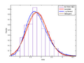
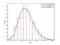
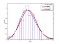
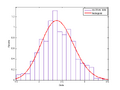
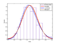
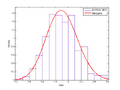
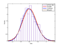
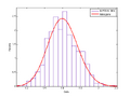
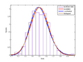
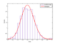
The least-squares data returned histograms with leftward-leaning "shoulders," which make sense given the preponderance of smaller slope in the total time period of the DJIA price:
With this in mind, fitting with known distributions seemed frivolous, but did provide elementary insight into the distribution fitting process in general. The log-likelihood rating given fits intrigues me in particular, but online resources are cryptic at best. Open science has not conquered this one just yet!
Examples of fits I tried on 500 iterations of average rates:
| 500 Iteration Probability Distribution
|
Fit Parameters
|
|
|
10 year:

Distribution:    Normal
Log likelihood:  -336.618
Domain:          -Inf < y < Inf
Mean:            2.79947
Variance:        0.225507

Parameter  Estimate  Std. Err.
mu          2.79947  0.0212371
sigma      0.474876  0.0150395

Estimated covariance of parameter estimates:
       mu            sigma
mu     0.000451013   -1.07538e-18
sigma  -1.07538e-18  0.000226185


Distribution:    Lognormal
Log likelihood:  -332.103
Domain:          0 < y < Inf
Mean:            2.79986
Variance:        0.231355

Parameter  Estimate  Std. Err.
mu          1.01503  0.00762697
sigma      0.170544  0.00540119

Estimated covariance of parameter estimates:
       mu            sigma
mu     5.81707e-05   -3.97263e-19
sigma  -3.97263e-19  2.91729e-05


Distribution:    Nakagami
Log likelihood:  -332.751
Domain:          0 < y < Inf
Mean:            2.79988
Variance:        0.222772

Parameter  Estimate  Std. Err.
mu         8.91723   0.553746
omega       8.0621   0.120739

Estimated covariance of parameter estimates:
       mu           omega
mu       0.306634   1.83823e-09
omega  1.83823e-09    0.014578
|
|
|
20 year:

Distribution:    Normal
Log likelihood:  -189.022
Domain:          -Inf < y < Inf
Mean:            2.41135
Variance:        0.124957

Parameter  Estimate  Std. Err.
mu          2.41135  0.0158086
sigma      0.353492  0.0111952

Estimated covariance of parameter estimates:
       mu           sigma
mu     0.000249913  2.0193e-19
sigma  2.0193e-19   0.000125333


Distribution:    Lognormal
Log likelihood:  -190.842
Domain:          0 < y < Inf
Mean:            2.41174
Variance:        0.13012

Parameter  Estimate  Std. Err.
mu         0.869288  0.00665194
sigma      0.148742   0.0047107

Estimated covariance of parameter estimates:
       mu           sigma
mu     4.42483e-05  2.60163e-21
sigma  2.60163e-21  2.21907e-05


Distribution:    Nakagami
Log likelihood:  -187.868
Domain:          0 < y < Inf
Mean:            2.41137
Variance:        0.124614

Parameter  Estimate  Std. Err.
mu         11.7865    0.735135
omega      5.93933   0.0773678

Estimated covariance of parameter estimates:
       mu           omega
mu       0.540424   2.95263e-09
omega  2.95263e-09  0.00598578
|
|
|
30 year:

Distribution:    Normal
Log likelihood:  6.36398
Domain:          -Inf < y < Inf
Mean:            1.90213
Variance:        0.0571925

Parameter  Estimate  Std. Err.
mu          1.90213   0.0106951
sigma      0.239149  0.00757394

Estimated covariance of parameter estimates:
       mu           sigma
mu     0.000114385  1.29821e-18
sigma  1.29821e-18  5.73646e-05


Distribution:    Lognormal
Log likelihood:  7.37713
Domain:          0 < y < Inf
Mean:            1.90226
Variance:        0.058345

Parameter  Estimate  Std. Err.
mu         0.635044  0.00565599
sigma      0.126472   0.0040054

Estimated covariance of parameter estimates:
       mu           sigma
mu     3.19902e-05  -1.3048e-19
sigma  -1.3048e-19  1.60432e-05


Distribution:    Nakagami
Log likelihood:  7.99048
Domain:          0 < y < Inf
Mean:            1.90219
Variance:        0.0568658

Parameter  Estimate  Std. Err.
mu         16.0294     1.00341
omega      3.67519   0.0410522

Estimated covariance of parameter estimates:
       mu           omega
mu        1.00684   2.23054e-09
omega  2.23054e-09  0.00168528
|
|
|
40 year:

Distribution:    Normal
Log likelihood:  191.058
Domain:          -Inf < y < Inf
Mean:            1.60399
Variance:        0.0273207

Parameter  Estimate  Std. Err.
mu         1.60399   0.00739199
sigma      0.16529   0.00523478

Estimated covariance of parameter estimates:
       mu            sigma
mu     5.46414e-05   -3.82513e-19
sigma  -3.82513e-19  2.74029e-05


Distribution:    Lognormal
Log likelihood:  191.951
Domain:          0 < y < Inf
Mean:            1.60404
Variance:        0.0276637

Parameter  Estimate  Std. Err.
mu          0.46718  0.00462479
sigma      0.103413  0.00327514

Estimated covariance of parameter estimates:
       mu            sigma
mu     2.13887e-05   -1.04169e-19
sigma  -1.04169e-19  1.07265e-05


Distribution:    Nakagami
Log likelihood:  192.237
Domain:          0 < y < Inf
Mean:            1.60402
Variance:        0.0271876

Parameter  Estimate  Std. Err.
mu         23.7815     1.49365
omega      2.60005   0.0238439

Estimated covariance of parameter estimates:
       mu           omega
mu        2.23098   2.58228e-09
omega  2.58228e-09  0.000568533
|
|
|
50 year:

Distribution:    Normal
Log likelihood:  316.326
Domain:          -Inf < y < Inf
Mean:            1.50232
Variance:        0.0165531

Parameter  Estimate  Std. Err.
mu          1.50232   0.0057538
sigma      0.128659  0.00407467

Estimated covariance of parameter estimates:
       mu            sigma
mu     3.31062e-05   -1.89468e-19
sigma  -1.89468e-19  1.66029e-05


Distribution:    Lognormal
Log likelihood:  317.216
Domain:          0 < y < Inf
Mean:            1.50234
Variance:        0.0166775

Parameter  Estimate   Std. Err.
mu          0.403344  0.00383718
sigma      0.0858019  0.00271737

Estimated covariance of parameter estimates:
       mu            sigma
mu     1.47239e-05   -4.44414e-20
sigma  -4.44414e-20  7.38411e-06


Distribution:    Nakagami
Log likelihood:  317.246
Domain:          0 < y < Inf
Mean:            1.50233
Variance:        0.0164799

Parameter  Estimate  Std. Err.
mu         34.3622      2.1628
omega      2.27348   0.0173446

Estimated covariance of parameter estimates:
       mu           omega
mu        4.67769   3.29831e-09
omega  3.29831e-09  0.000300836
|
Thoughts
This lab basically turned into a large exercise on data manipulation and information-hunting. I also was able to combine concepts from lecture on linear least-squares fitting with more general error propagation.
The distribution analysis is gratifying in that I see a reflection in the processed data corresponding to trends in the raw data. Something to try regarding the distribution fit would be to generate a fake DJIA from the best-fit distribution function and compare with the real data. I imagine this would involve something like executing our lab process in reverse, generating huge numbers of linear windows with random start dates and distribution-derived slopes. One could then "smooth" all these disjointed, overlapping linear sections into a fake DJIA.