User:Alexander T. J. Barron/Notebook/PHYC 307L Lab Notebook/finance notes

Day 1

^{SJK 16:40, 19 December 2008 (EST)}

16:40, 19 December 2008 (EST)
Hey Der, This looks really great, and I am really looking forward to looking at it some more. Sorry about the huge delay in me looking at it, but I hope to look at it some more after the semester grading is done. Thanks for taking on this project!

The topics of this lab were unbounded, so most of the work was in trying to narrow our project to a realizable goal. After exploring some deeper topics that led down unanswerable (and endless) philosophical and political paths we decided we must narrow our search. So we decided to set some goals, then choose a topic of finance that would lead to valuable exercises in the following:

• data analysis
• computational technique
• finance terminology
• historical perspective

We remembered a lab we did in PHYS 290 with Dr. Stephen Boyd where we analyzed stock data. We loaded said data to MATAB, then performed simple and exponential moving averages on it. This excercise gave us a bit of inspiration, or rather helped us to focus our topic search. After contacting Dr. Boyd about the source of his stock data, and discussing with Dr. Koch, our goal then eventually became the following:

Purpose of Our Finance lab

The purpose of this lab is to study rate growth in the stock market, we will do this by asking a question.

If one makes a ten year investment in the stock market, what should one expect, based on historical analysis, to be one's rate of growth?

Questions that come about from this question:

• What financial data/market would be a good indicator for such a broad question?
• Where do we get this data?
• How do we simulate "investment" with the historical data in hand?
• What does it mean to expect a rate of growth?
• Is there an average rate of growth, or maybe even a rate that fits some known distribution?

What we learned on the way

What we learned from our initial exploration:

Financial gurus have created market indicators called "indices" to chart the progress of sectors of the stock market. Well known market indices are the NASDAQ, the S&P 500, and the Dow Jones. A stock index is basically a summation of the stocks of a selected group of companies. The selection of course is chosen based on the purpose of the index, to follow a certain industry within the ecomomy.

We learned that these indices are created using two different methods:

• Price weighted: is just the average of the prices of all the stocks making up the index. An example is the Dow Jones Industrial Average which is a simple summation of the prices divided by the Dow jones "divisor", the number of component companies. In this way it is a true average.

[math]\displaystyle{ \text{DJIA} = {\sum p \over d}, }[/math]

where p is the price of the shares and d is the # of companies.

• Market value-weighted: accounts for the size of each company making up the index such that price changes in smaller companies don't effect the index more than they should as compared to the bigger companies.

We found these methods very interesting and spent a considerable amount of time exploring this as a possible purpose of our lab. We considered making our own indices for fun, or making an index that would capture the trends of the recent financial crisis. We decided that this would be unnecessary and that we should use the indices already out there.

Another idea we pursued was calculation of net present value, and the comparison of investments at different times. We researched into net present value, with the idea in mind that we will calculate the true value of investing in US Treasury bonds over a period of time.

Net present value (NPV) is a comparison of a dollar today to a projected value for the same dollar at some point in the future. Present value is the value on a given date of a future payment or series of future payments, discounted to reflect the time value of money and other factors such as investment risk. A common model of present value is the compund interest formula that calculates how much money you will have in an account make a certain interest after a certain amount of time.

This led us to bonds. Maybe we could compare bonds with savings accounts, or other securities like stock. We ended up learning a little about bonds...

A bond is a loan in the form of a security. A security is defined as something fungible (exhangeable with itself like currency, oil, gold). However, a bond is not an equity like stock. Some bond vocabulary we learned:

• principle/nominal/face value: the ammount which the issuer pays interest, which has to be repaid in the end.
• issue price: the price the investor buys the bond when issued.
• maturity date: the time the issuer repays the nominal amount.
• yield: percent that measures cash return to owners of the bond.
• nominal yield: yearly total of interest paid to owner divided by principal face value of bond.

We might use our new knowledge of bonds and compare bonds yield rates to the average growth rate fo the stock market. Which is a higher growth investment? Obviously, this is a complicated question. The stock market may grow faster, but it falls faster too and is high risk compared to bonds (especially US treasury bonds). Therefore comparing stock to bonds is sort of silly but might prove to be a worthwhile comparison.

Day 2

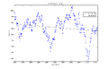
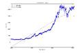
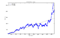
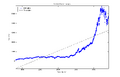
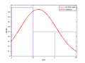
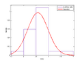
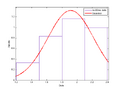
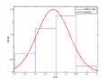
We were still somewhat adrift regarding real lab-worthy content of our lab, so we leapt at Dr. Koch's idea to analyze randomly-generated time windows over the course of the DJIA. We initially chose 10-year windows in order to compare to a 10-year US security bond. When creating the code to do this, we ended up discussing whether we should take least-squares fits of each window, or to take 10-year "snapshots," which find the slope from the two stock prices at the endpoints of the window. Snapshots make sense in that a person investing during that exact time period would see exactly that rate of growth. Least-squares fits show more of a trend over the 10 years, so that someone who invested only 9 years, 10 months might see growth closer to the fit than the snapshot.

The code I generated on that day basically failed - I was tearing my hair out for a while, but I got it eventually. I ended up generating data for 10-, 20-, 30-, 40-, and 50-year windows, all with 100 randomly-generated iterations. My hypothesis is that the shorter windows will be more sensitive to small changes in the market, so their slopes will be more severe. Ideally, the number of iterations should be inversely proportional to the length of the window because the longer windows will naturally cover more data than the shorter. However, equal iteration counts make easier analysis.

Data Analysis

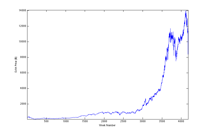
Data from Yahoo! Finance.

Ticker: ^DJI, weekly from 10/01/1928 to 10/27/08.

Using the least-squares fit provides a great opportunity to hone my error propagation skills (proven quite dull in my last attempt). SO!.... here is the rundown:

Each window will have an error according to these parameters, from the line-fitting help page:

[math]\displaystyle{ \ y=A+Bx }[/math]

[math]\displaystyle{ \sigma_B^2 = N \frac{\sigma_y^2}{\Delta_{fixed}} }[/math]

(I believe this is the same as 1/N * σ_y² / σ_x², where σ_x² is the population variance of the experimental x values, not the variance of an individual x measurement.)

Since there is no error on the stock price measurements every week, I'll have to find the inferred error:

[math]\displaystyle{ \sigma_{y~inferred} =\sqrt{\frac {1}{N-2} \sum (y_i - A - Bx_i)^2} }[/math] [math]\displaystyle{ \mbox{,}~~~~~~~\mbox{recall,}~~ \chi^2 = \frac {1}{\sigma_y^2} \sum (y_i - A - Bx_i)^2 }[/math]

[math]\displaystyle{ \Delta_{fixed}=N \sum x_i^2 - \left ( \sum x_i \right )^2 }[/math] (This is actually N² times the population variance of x...not sure if that helps in any kind of understanding, though.)

In my code, I utilized the above note on Δ_fixed.

To find the error on the mean of all 100 slope measurements, I use the linear-approximation method and add in quadrature:

[math]\displaystyle{ r_{avg} = \frac{1}{T} \times (r_1 + r_2 + ... +r_T) \longrightarrow \sigma_{r_{avg}} = \sqrt{(\frac{\partial r_{avg}}{\partial r_1} \sigma_{r_1})^2 + (\frac{\partial r_{avg}}{\partial r_2} \sigma_{r_2})^2 + ... + (\frac{\partial r_{avg}}{\partial r_T} \sigma_{r_T})^2} , }[/math]

[math]\displaystyle{ T = 100, \sigma_B \rightarrow \sigma_i }[/math]

[math]\displaystyle{ \downarrow }[/math]

[math]\displaystyle{ \sigma_{r_{avg}} = \frac{1}{100}\sqrt{{\sigma_{r_1}}^2 + {\sigma_{r_2}}^2 + ... + {\sigma_{r_T}}^2} }[/math]

Slope Data [$/week] ± σravg	Sample Window
10 Year Window 1) 2.4689 ± 0.0007 11) 2.6043 ± 0.0007 2) 3.1063 ± 0.0011 12) 3.2287 ± 0.0011 3) 2.5977 ± 0.0008 13) 2.1363 ± 0.0009 4) 2.4893 ± 0.0007 14) 2.8116 ± 0.0008 5) 2.8451 ± 0.0007 15) 2.3922 ± 0.0005 6) 2.1571 ± 0.0007 16) 2.7420 ± 0.0009 7) 3.0676 ± 0.0009 17) 3.1118 ± 0.0008 8) 3.4700 ± 0.0009 18) 2.4796 ± 0.0009 9) 2.1050 ± 0.0006 19) 2.3554 ± 0.0009 10) 2.2250 ± 0.0008 20) 2.0223 ± 0.0009
20 Year Window 1) 2.9810 ± 0.0003 11) 2.5314 ± 0.0003 2) 2.8751 ± 0.0004 12) 2.5233 ± 0.0003 3) 2.1529 ± 0.0003 13) 2.0260 ± 0.0003 4) 2.5026 ± 0.0002 14) 2.8666 ± 0.0003 5) 2.3646± 0.0002 15) 2.8161 ± 0.0003 6) 3.5018 ± 0.0004 16) 2.0481 ± 0.0003 7) 2.3696 ± 0.0002 17) 2.8723 ± 0.0003 8) 2.7557 ± 0.0003 18) 2.6072 ± 0.0003 9) 2.0702 ± 0.0003 19) 3.0362 ± 0.0004 10) 2.6607 ± 0.0003 20) 1.8809 ± 0.0003
30 Year Window 1) 1.6386 ± 0.0002 11) 1.7714 ± 0.0002 2) 1.6168 ± 0.0002 12) 1.9832 ± 0.0002 3) 1.9087 ± 0.0002 13) 1.7668 ± 0.0002 4) 1.4801 ± 0.0002 14) 1.2027 ± 0.0002 5) 1.8070 ± 0.0002 15) 2.0399± 0.0002 6) 2.3613 ± 0.0002 16) 1.9900 ± 0.0002 7) 1.9316 ± 0.0002 17) 2.1310 ± 0.0002 8) 2.3433 ± 0.0002 18) 2.3271 ± 0.0002 9) 2.1834 ± 0.0002 19) 2.1681 ± 0.0002 10) 1.6845 ± 0.0002 20) 1.9814 ± 0.0002
40 Year Window 1) 1.2491 ± 0.0002 11) 1.5066 ± 0.0002 2) 1.6391 ± 0.0002 12) 1.6332 ± 0.0002 3) 1.4006 ± 0.0002 13) 1.7675 ± 0.0002 4) 1.6526 ± 0.0001 14) 1.7078 ± 0.0002 5) 1.8456 ± 0.0002 15) 1.4713 ± 0.0002 6) 1.4773 ± 0.0002 16) 1.6195 ± 0.0002 7) 1.5594 ± 0.0001 17) 1.6892 ± 0.0002 8) 1.5667 ± 0.0002 18) 1.5924 ± 0.0002 9) 1.6973 ± 0.0001 19) 1.7595 ± 0.0002 10) 1.3066 ± 0.0002 20) 1.3776 ± 0.0002
50 Year Window 1) 1.5937 ± 0.0001 11) 1.4359 ± 0.0002 2) 1.3238 ± 0.0002 12) 1.4196 ± 0.0002 3) 1.5460 ± 0.0001 13) 1.5010 ± 0.0001 4) 1.4301 ± 0.0002 14) 1.6835 ± 0.0002 5) 1.4891 ± 0.0002 15) 1.4429 ± 0.0001 6) 1.3474 ± 0.0001 16) 1.4743 ± 0.0001 7) 1.6312 ± 0.0002 17) 1.4178 ± 0.0001 8) 1.4696 ± 0.0002 18) 1.5034 ± 0.0002 9) 1.5794 ± 0.0001 19) 1.4420 ± 0.0001 10) 1.3559 ± 0.0001 20) 1.3633 ± 0.0001

My gut is telling me that my error is off-base once again, but I don't see a flaw in my approach based on Dr. Koch's lectures and reference to Taylor.

Distribution?

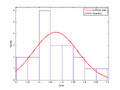
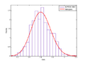
My original plan was to fit probability-density plots with various distributions, Gaussian chief among them. Here are the results for each time window, 20 trials:

20 Iteration Probability Distribution	Fit Parameters
10-year ravg Distribution	10 year: Distribution: Normal Log likelihood: -10.3216 Domain: -Inf < y < Inf Mean: 2.62082 Variance: 0.172784 Parameter Estimate Std. Err. mu 2.62082 0.0929472 sigma 0.415672 0.0683361 Estimated covariance of parameter estimates: mu sigma mu 0.00863918 9.85064e-18 sigma 9.85064e-18 0.00466983
20-year ravg Distribution	20 year: Distribution: Normal Log likelihood: -10.0321 Domain: -Inf < y < Inf Mean: 2.57211 Variance: 0.167852 Parameter Estimate Std. Err. mu 2.57211 0.0916112 sigma 0.409698 0.0673539 Estimated covariance of parameter estimates: mu sigma mu 0.00839261 -6.54755e-18 sigma -6.54755e-18 0.00453655
30-year ravg Distribution	30 Year: Distribution: Normal Log likelihood: -3.94363 Domain: -Inf < y < Inf Mean: 1.91585 Variance: 0.0913083 Parameter Estimate Std. Err. mu 1.91585 0.0675678 sigma 0.302173 0.0496769 Estimated covariance of parameter estimates: mu sigma mu 0.00456541 -1.50689e-18 sigma -1.50689e-18 0.00246779
40-year ravg Distribution	40 Year: Distribution: Normal Log likelihood: 8.93404 Domain: -Inf < y < Inf Mean: 1.57594 Variance: 0.0251907 Parameter Estimate Std. Err. mu 1.57594 0.0354899 sigma 0.158716 0.0260927 Estimated covariance of parameter estimates: mu sigma mu 0.00125953 -1.75362e-18 sigma -1.75362e-18 0.000680829
50-year ravg Distribution	50 year: Distribution: Normal Log likelihood: 18.8652 Domain: -Inf < y < Inf Mean: 1.47248 Variance: 0.00933117 Parameter Estimate Std. Err. mu 1.47248 0.0216 sigma 0.096598 0.0158806 Estimated covariance of parameter estimates: mu sigma mu 0.000466558 -2.79991e-19 sigma -2.79991e-19 0.000252194

I think it is fairly obvious I need much more data to get an accurate picture of the distribution. Here goes for 500 trials:

500 Iteration Probability Distribution	Fit Parameters
10-year ravg Distribution Best: Log Normal	10 year: Distribution: Normal Log likelihood: -336.618 Domain: -Inf < y < Inf Mean: 2.79947 Variance: 0.225507 Parameter Estimate Std. Err. mu 2.79947 0.0212371 sigma 0.474876 0.0150395 Estimated covariance of parameter estimates: mu sigma mu 0.000451013 -1.07538e-18 sigma -1.07538e-18 0.000226185 Distribution: Lognormal Log likelihood: -332.103 Domain: 0 < y < Inf Mean: 2.79986 Variance: 0.231355 Parameter Estimate Std. Err. mu 1.01503 0.00762697 sigma 0.170544 0.00540119 Estimated covariance of parameter estimates: mu sigma mu 5.81707e-05 -3.97263e-19 sigma -3.97263e-19 2.91729e-05 Distribution: Nakagami Log likelihood: -332.751 Domain: 0 < y < Inf Mean: 2.79988 Variance: 0.222772 Parameter Estimate Std. Err. mu 8.91723 0.553746 omega 8.0621 0.120739 Estimated covariance of parameter estimates: mu omega mu 0.306634 1.83823e-09 omega 1.83823e-09 0.014578
20-year ravg Distribution Best: Nakagami	20 year: Distribution: Normal Log likelihood: -189.022 Domain: -Inf < y < Inf Mean: 2.41135 Variance: 0.124957 Parameter Estimate Std. Err. mu 2.41135 0.0158086 sigma 0.353492 0.0111952 Estimated covariance of parameter estimates: mu sigma mu 0.000249913 2.0193e-19 sigma 2.0193e-19 0.000125333 Distribution: Lognormal Log likelihood: -190.842 Domain: 0 < y < Inf Mean: 2.41174 Variance: 0.13012 Parameter Estimate Std. Err. mu 0.869288 0.00665194 sigma 0.148742 0.0047107 Estimated covariance of parameter estimates: mu sigma mu 4.42483e-05 2.60163e-21 sigma 2.60163e-21 2.21907e-05 Distribution: Nakagami Log likelihood: -187.868 Domain: 0 < y < Inf Mean: 2.41137 Variance: 0.124614 Parameter Estimate Std. Err. mu 11.7865 0.735135 omega 5.93933 0.0773678 Estimated covariance of parameter estimates: mu omega mu 0.540424 2.95263e-09 omega 2.95263e-09 0.00598578
30-year ravg Distribution Best: Nakagami	30 year: Distribution: Normal Log likelihood: 6.36398 Domain: -Inf < y < Inf Mean: 1.90213 Variance: 0.0571925 Parameter Estimate Std. Err. mu 1.90213 0.0106951 sigma 0.239149 0.00757394 Estimated covariance of parameter estimates: mu sigma mu 0.000114385 1.29821e-18 sigma 1.29821e-18 5.73646e-05 Distribution: Lognormal Log likelihood: 7.37713 Domain: 0 < y < Inf Mean: 1.90226 Variance: 0.058345 Parameter Estimate Std. Err. mu 0.635044 0.00565599 sigma 0.126472 0.0040054 Estimated covariance of parameter estimates: mu sigma mu 3.19902e-05 -1.3048e-19 sigma -1.3048e-19 1.60432e-05 Distribution: Nakagami Log likelihood: 7.99048 Domain: 0 < y < Inf Mean: 1.90219 Variance: 0.0568658 Parameter Estimate Std. Err. mu 16.0294 1.00341 omega 3.67519 0.0410522 Estimated covariance of parameter estimates: mu omega mu 1.00684 2.23054e-09 omega 2.23054e-09 0.00168528
40-year ravg Distribution Best: Nakagami	40 year: Distribution: Normal Log likelihood: 191.058 Domain: -Inf < y < Inf Mean: 1.60399 Variance: 0.0273207 Parameter Estimate Std. Err. mu 1.60399 0.00739199 sigma 0.16529 0.00523478 Estimated covariance of parameter estimates: mu sigma mu 5.46414e-05 -3.82513e-19 sigma -3.82513e-19 2.74029e-05 Distribution: Lognormal Log likelihood: 191.951 Domain: 0 < y < Inf Mean: 1.60404 Variance: 0.0276637 Parameter Estimate Std. Err. mu 0.46718 0.00462479 sigma 0.103413 0.00327514 Estimated covariance of parameter estimates: mu sigma mu 2.13887e-05 -1.04169e-19 sigma -1.04169e-19 1.07265e-05 Distribution: Nakagami Log likelihood: 192.237 Domain: 0 < y < Inf Mean: 1.60402 Variance: 0.0271876 Parameter Estimate Std. Err. mu 23.7815 1.49365 omega 2.60005 0.0238439 Estimated covariance of parameter estimates: mu omega mu 2.23098 2.58228e-09 omega 2.58228e-09 0.000568533
50-year ravg Distribution Best: Nakagami	50 year: Distribution: Normal Log likelihood: 316.326 Domain: -Inf < y < Inf Mean: 1.50232 Variance: 0.0165531 Parameter Estimate Std. Err. mu 1.50232 0.0057538 sigma 0.128659 0.00407467 Estimated covariance of parameter estimates: mu sigma mu 3.31062e-05 -1.89468e-19 sigma -1.89468e-19 1.66029e-05 Distribution: Lognormal Log likelihood: 317.216 Domain: 0 < y < Inf Mean: 1.50234 Variance: 0.0166775 Parameter Estimate Std. Err. mu 0.403344 0.00383718 sigma 0.0858019 0.00271737 Estimated covariance of parameter estimates: mu sigma mu 1.47239e-05 -4.44414e-20 sigma -4.44414e-20 7.38411e-06 Distribution: Nakagami Log likelihood: 317.246 Domain: 0 < y < Inf Mean: 1.50233 Variance: 0.0164799 Parameter Estimate Std. Err. mu 34.3622 2.1628 omega 2.27348 0.0173446 Estimated covariance of parameter estimates: mu omega mu 4.67769 3.29831e-09 omega 3.29831e-09 0.000300836

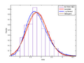
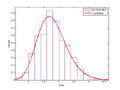
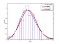
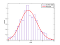
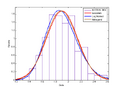
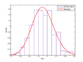
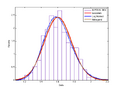
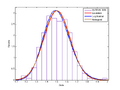
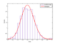
I chose the "best" fit from the log-likelihood value. Internet resources are almost all entirely cryptic regarding this quantity, but I believe that a higher value indicates a better fit. However, just eyeballing would suggest that I either need more iterations to truly analyze the data, or that none of the distributions correlate very well. Specifically, the larger-window averages seem to have "flat-topped" histograms, which none of the distributions provided models. There is an observable trend in the leftward-leaning "shoulder" of each histogram, which basically makes a Gaussian distribution out of the question. Both Nakagami and Log Normal take this lean into account. In truth, I think running thousands of iterations would give clearer results and take away the hills and valleys still prevalent in each histogram. Unfortunately, MATLAB has revealed its lack of speed to me- 10,000 iterations would take days to run.

Although I can fit these histograms marginally well with a known distribution, I don't think this means anything in a fundamental sense. According to Wikipedia, Nakagami created his distribution to analyze radio signals in his research, so comparing it with these histograms is frivolous. If one looks at the entire history of the DJIA used in this lab, lower slope dominates, correlating to the leftward-leaning shoulder on the histogram. It is gratifying, however, that I see a reflection in the processed data corresponding to what is evident in the raw data.

Code

%% Finance Lab

% Alexander Barron
% Junior Lab Fall 2008

close all, clear all;

%% Load Data

DJIAprice = csvread('DJIA28to03weekly.csv',1,6,[1 6 4177 6]);
DJIAprice = flipud(DJIAprice);
DJIAprice = DJIAprice.';

t = linspace(1,length(DJIAprice),length(DJIAprice));

% scrsz = get(0,'ScreenSize');
% figure('Position',[1 scrsz(4)/1.5 scrsz(3)/1.55 scrsz(4)/1.6]);
% 
% plot(t,DJIAprice);
% axis tight;
% xlabel('Week Number');
% ylabel('DJIA Price [$]');


%% 20 Iterations

rav10vec = zeros(1,20);
rav20vec = zeros(1,20);
rav30vec = zeros(1,20);
rav40vec = zeros(1,20);
rav50vec = zeros(1,20);

rav10errvec = zeros(1,20);
rav20errvec = zeros(1,20);
rav30errvec = zeros(1,20);
rav40errvec = zeros(1,20);
rav50errvec = zeros(1,20);

for f=1:100;

    %% 10-year windows

    for j=1:100;

        windstart10 = ceil(rand*(length(t)-520));
        windend10 = windstart10 + 519;
        windt10{j} = linspace(windstart10,windend10,520);   % cell structure of 
                                                            % randomly-
                                                            % generated 10-year
                                                            % time windows
        windval10{j} = DJIAprice(windt10{j});
        [linfit10{j},linfit10err{j}] = polyfit(windt10{j},windval10{j},1);
        linval10{j} = linfit10{j}(1).*windt10{j}+linfit10{j}(2);


        clear windstart10, clear windend10;

    end


    % figure('Position',[20 scrsz(4)/1.5 scrsz(3)/1.55 scrsz(4)/1.6]);
    % randind=ceil(100*rand);
    % plot(windt10{randind},windval10{randind},'b.');
    % hold on;
    % plot(windt10{randind},linval10{randind},'k--');
    % axis tight;
    % legend('DJIA price','Trend Line','Location','Best');
    % title('10-year Window Example');
    % ylabel('DJIA price');
    % xlabel('Week Number');


    %% 20-year windows

    for j=1:100;

        windstart20 = ceil(rand*(length(t)-1040));
        windend20 = windstart20 + 1039;
        windt20{j} = linspace(windstart20,windend20,1040);      


        windval20{j} = DJIAprice(windt20{j});
        [linfit20{j},linfit20err{j}] = polyfit(windt20{j},windval20{j},1);
        linval20{j} = linfit20{j}(1).*windt20{j}+linfit20{j}(2);


        clear windstart20, clear windend20;

    end


    % figure('Position',[40 scrsz(4)/1.5 scrsz(3)/1.55 scrsz(4)/1.6]);
    % randind2=ceil(100*rand);
    % plot(windt20{randind2},windval20{randind2},'b.');
    % hold on;
    % plot(windt20{randind2},linval20{randind2},'k--');
    % axis tight;
    % legend('DJIA price','Trend Line','Location','Best');
    % title('20-year Window Example');
    % ylabel('DJIA price');
    % xlabel('Week Number');


    %% 30-year windows

    for j=1:100;

        windstart30 = ceil(rand*(length(t)-1560));
        windend30 = windstart30 + 1559;
        windt30{j} = linspace(windstart30,windend30,1560);         


        windval30{j} = DJIAprice(windt30{j});
        [linfit30{j},linfit30err{j}] = polyfit(windt30{j},windval30{j},1);
        linval30{j} = linfit30{j}(1).*windt30{j}+linfit30{j}(2);


        clear windstart30, clear windend30;

    end


    % figure('Position',[60 scrsz(4)/1.5 scrsz(3)/1.55 scrsz(4)/1.6]);
    % randind3=ceil(100*rand);
    % plot(windt30{randind3},windval30{randind3},'b.');
    % hold on;
    % plot(windt30{randind3},linval30{randind3},'k--');
    % axis tight;
    % legend('DJIA price','Trend Line','Location','Best');
    % title('30-year Window Example');
    % ylabel('DJIA price');
    % xlabel('Week Number');


    %% 40-year windows

    for j=1:100;

        windstart40 = ceil(rand*(length(t)-2080));
        windend40 = windstart40 + 2079;
        windt40{j} = linspace(windstart40,windend40,2080);         


        windval40{j} = DJIAprice(windt40{j});
        [linfit40{j},linfit40err{j}] = polyfit(windt40{j},windval40{j},1);
        linval40{j} = linfit40{j}(1).*windt40{j}+linfit40{j}(2);


        clear windstart40, clear windend40;

    end


    % figure('Position',[80 scrsz(4)/1.5 scrsz(3)/1.55 scrsz(4)/1.6]);
    % randind4=ceil(100*rand);
    % plot(windt40{randind4},windval40{randind4},'b.');
    % hold on;
    % plot(windt40{randind4},linval40{randind4},'k--');
    % axis tight;
    % legend('DJIA price','Trend Line','Location','Best');
    % title('40-year Window Example');
    % ylabel('DJIA price');
    % xlabel('Week Number');


    %% 50-year windows

    for j=1:100;

        windstart50 = ceil(rand*(length(t)-2600));
        windend50 = windstart50 + 2599;
        windt50{j} = linspace(windstart50,windend50,2600);    


        windval50{j} = DJIAprice(windt50{j});
        [linfit50{j},linfit50err{j}] = polyfit(windt50{j},windval50{j},1);
        linval50{j} = linfit50{j}(1).*windt50{j}+linfit50{j}(2);


        clear windstart50, clear windend50;

    end


    % figure('Position',[80 scrsz(4)/1.5 scrsz(3)/1.55 scrsz(4)/1.6]);
    % randind5=ceil(100*rand);
    % plot(windt50{randind5},windval50{randind5},'b.');
    % hold on;
    % plot(windt50{randind5},linval50{randind5},'k--');
    % axis tight;
    % legend('DJIA price','Trend Line','Location','Best');
    % title('50-year Window Example');
    % ylabel('DJIA price');
    % xlabel('Week Number');


    %% Slope Mean

    slopevec10 = zeros(1,100);
    slopevec20 = zeros(1,100);
    slopevec30 = zeros(1,100);
    slopevec40 = zeros(1,100);
    slopevec50 = zeros(1,100);

    for j=1:100;

        slopevec10(j) = linfit10{j}(1);
        slopevec20(j) = linfit20{j}(1);
        slopevec30(j) = linfit30{j}(1);
        slopevec40(j) = linfit40{j}(1);
        slopevec50(j) = linfit50{j}(1);

    end;

    rav10vec(f) = mean(slopevec10)
    rav20vec(f) = mean(slopevec20);
    rav30vec(f) = mean(slopevec30);
    rav40vec(f) = mean(slopevec40);
    rav50vec(f) = mean(slopevec50);


    %% Error Propogation

    % inferred error for each fit...this is huge...

    deg10 = linfit10err{j}.df;      % degrees of freedom for each window
    deg20 = linfit20err{j}.df;
    deg30 = linfit30err{j}.df;
    deg40 = linfit40err{j}.df;
    deg50 = linfit50err{j}.df;

    degsigstart = 0;        % representing sigma inferred times d. o. f.
                            % and setting up for sum of chi^2*sigy^2       

    degsig10 = zeros(1,100);
    degsig20 = zeros(1,100);
    degsig30 = zeros(1,100);
    degsig40 = zeros(1,100);
    degsig50 = zeros(1,100);

    deltafixed10 = zeros(1,100);
    deltafixed20 = zeros(1,100);
    deltafixed30 = zeros(1,100);
    deltafixed40 = zeros(1,100);
    deltafixed50 = zeros(1,100);

    for j=1:100;        % accessing all above structures for necessary data
                        % to properly propogate a plethora of faux pas
                        % (errors...)
        for k=1:520;    
            degsig10(j) = degsigstart +...      % sum of chi^2*sigy^2
                (windval10{j}(k) - linfit10{j}(2) - linfit10{j}(1)*windt10{j}(k))^2;
        end;

        deltafixed10(j) = 520*(519)*var(windt10{j});  % correcting MATLAB's version
                                                      % of population variance
        for k=1:1040;
            degsig20(j) = degsigstart +...
                (windval20{j}(k) - linfit20{j}(2) - linfit20{j}(1)*windt20{j}(k))^2;
        end;

        deltafixed20(j) = 1040*(1039)*var(windt20{j});

        for k=1:1560;
            degsig30(j) = degsigstart +...
                (windval30{j}(k) - linfit30{j}(2) - linfit30{j}(1)*windt30{j}(k))^2;
        end;

        deltafixed30(j) = 1560*(1559)*var(windt30{j});

        for k=1:2080;
            degsig40(j) = degsigstart +...
                (windval40{j}(k) - linfit40{j}(2) - linfit40{j}(1)*windt40{j}(k))^2;
        end;

        deltafixed40(j) = 2080*(2079)*var(windt40{j});

        for k=1:2600;
            degsig50(j) = degsigstart +...
                (windval50{j}(k) - linfit50{j}(2) - linfit50{j}(1)*windt50{j}(k))^2;
        end;

        deltafixed50(j) = 2600*(2599)*var(windt50{j});

    end;

    sigpinf10 = sqrt(degsig10./deg10);
    sigpinf20 = sqrt(degsig20./deg20);
    sigpinf30 = sqrt(degsig30./deg30);
    sigpinf40 = sqrt(degsig40./deg40);
    sigpinf50 = sqrt(degsig50./deg50);

    ratesig10 = sqrt(520.*sigpinf10.^2./deltafixed10);
    ratesig20 = sqrt(1040.*sigpinf20.^2./deltafixed20);
    ratesig30 = sqrt(1560.*sigpinf30.^2./deltafixed30);
    ratesig40 = sqrt(2080.*sigpinf40.^2./deltafixed40);
    ratesig50 = sqrt(2600.*sigpinf50.^2./deltafixed50);

    rav10errvec(f) = (1/100).*sqrt(sum(ratesig10.^2));  % adding error contributions
    rav20errvec(f) = (1/100).*sqrt(sum(ratesig20.^2));  % of 100 slope fits in 
    rav30errvec(f) = (1/100).*sqrt(sum(ratesig30.^2));  % quadrature
    rav40errvec(f) = (1/100).*sqrt(sum(ratesig40.^2));
    rav50errvec(f) = (1/100).*sqrt(sum(ratesig50.^2));

end;