Open writing projects/Sage and cython a brief introduction

|
This page is part of the Open Writing Project Sage_and_cython_a_brief_introduction. (More Open Writing Projects.) |
Author: Marshall Hampton
Sage and Cython: a brief introduction
Abstract
This is a quick introduction to Sage, a powerful new computational platform that builds on the strengths of Python. This article was directly inspired by Julius B. Lucks' "Python: All A Scientist Needs"; I recommend reading it first as it explains some of the attractions of Python and biopython. One thing I will highlight is using Cython[1] in Sage to make very fast code in an easy way.
Sage is a free and open-source project for computation of all sorts that uses Python as its primary language and "glue". One of the goals of Sage is to provide a viable free and open-source alternative to Matlab, Maple, and Mathematica. Sage unifies a great deal of open-source mathematical and statistical software; it includes biopython as an optional package and the statistics language R by default.
Sage notebook interface
A key feature of Sage is its notebook web-browser interface.
Jose Unpingco has made a good short introductory video on the notebook interface that may help get a sense of what its like.
These videos made by Dr. Jose Unpingco Attribution 3.0 license.
Introduction.
<html>
<object id="csSWF" classid="clsid:d27cdb6e-ae6d-11cf-96b8-444553540000" width="640" height="498" codebase="http://active.macromedia.com/flash7/cabs/ swflash.cab#version=9,0,28,0">
               <param name="src" value="sageIntroClean.swf"/>
               <param name="bgcolor" value="#1a1a1a"/>
               <param name="quality" value="best"/>
               <param name="allowScriptAccess" value="always"/>
               <param name="allowFullScreen" value="true"/>
               <param name="scale" value="showall"/>
               <param name="flashVars" value="autostart=false"/>
               <embed name="csSWF" src="http://sage.math.washington.edu/home/wdj/expository/unpingco/sageIntroClean.swf" width="640" height="498" bgcolor="#1a1a1a" quality="best" allowScriptAccess="always" allowFullScreen="true" scale="showall" flashVars="autostart=false" pluginspage="http://www.macromedia.com/shockwave/download/index.cgi?P1_Prod_Version=ShockwaveFlash">
</embed> </object> </html>
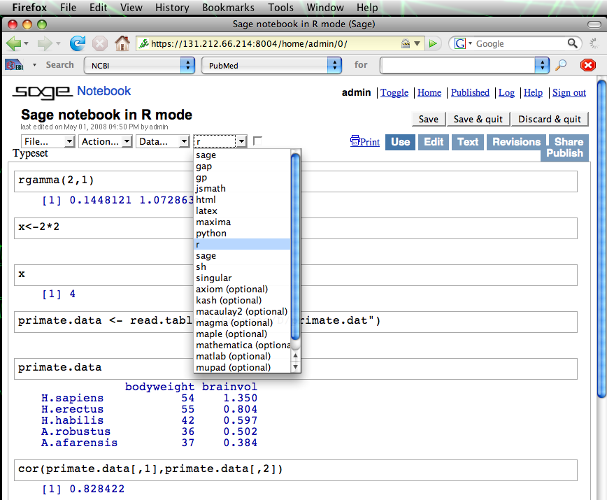
The notebook starts by default in native Sage mode, which is almost identical to python. However, other environments are available. The screenshot below shows a Sage notebook in R mode, with some simple R commands executed [2].
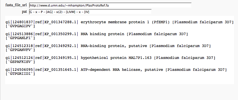
The @interact command in the Sage notebook provides an easy way to make simple GUIs to explore data. In the example below, a user can enter the URL of a fasta-formatted protein file and a PROSITE-style regular expression. Using biopython and the "re" module of python we can search for and display matches to the pattern. For this screenshot, I used proteins from the malaria-causing Plasmodium falciparum and a fragment of the transthyretin pattern (Prosite PS00768). This is just for illustrative purposes - I do not claim any significance for these matches.
def PStoRE(PrositePattern):
   """
   Converts a PROSITE regular expression to a python r.e.
   """
   rePattern = PrositePattern
   rePattern = rePattern.replace('-',)
   rePattern = rePattern.replace(' ',)
   rePattern = rePattern.replace('x','.')
   rePattern = rePattern.replace('{','[^')
   rePattern = rePattern.replace('}',']')
   rePattern = rePattern.replace('(','{')
   rePattern = rePattern.replace(')','}')
   return rePattern
from Bio import Fasta
import re
import urllib2 as U
@interact
def re_scan(fasta_file_url = 'http://www.d.umn.edu/~mhampton/PlasProtsRef.fa', pat = input_box('G - x - P - [AG] - x(2) - [LIVM] - x - [IV] ', type = str, width = 60)):
   re_pat = re.compile(PStoRE(pat))
   parser = Fasta.RecordParser()
   prot_file = U.urlopen(fasta_file_url)
   fasta_iterator = Fasta.Iterator(prot_file, parser = parser)
   for record in fasta_iterator:
       matches = re_pat.findall(record.sequence)
       if len(matches) != 0:
           html(record.title)
           html(matches)
           print
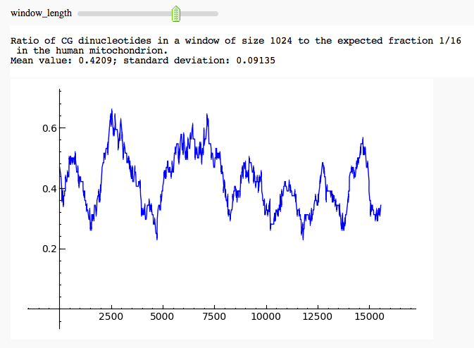
Here is another example of the interact command, along with some of Sage's 2D plotting. We take a human mitochondrial DNA sequence and plot the fraction of CG dinucleotides in a window of variable size. This fraction is divided by 16, to normalize it against the expected value in the case of independently, uniformly distributed nucleotides (obviously a simple model in this case).
from Bio import SeqIO
import urllib2 as U
import scipy.stats as Stat
f = U.urlopen('http://www.d.umn.edu/~mhampton/HomoSmito.fa')
p = SeqIO.parse(f, 'fasta')
hsmito = p.next().seq.tostring()
f.close()
display_f = RealField(16)
@interact
def cgplot(window_length = slider([2^i for i in range(4,12)],default = 2^9)):
   avg = [16.0*hsmito[x-window_length: x+window_length].count('CG')/(2*window_length-1) for x in range(window_length, len(hsmito) - window_length)]
   mean = display_f(Stat.mean(avg))
   std = display_f(Stat.std(avg))
   html('Ratio of CG dinucleotides in a window of size ' + str(2*window_length) + ' to the expected fraction 1/16
 in the human mitochondrion.
Mean value: ' + str(mean) + '; standard deviation: ' + str(std))
   show(list_plot(avg, plotjoined=True), ymin = 0, ymax = max(avg))
For more (mostly mathematical) examples of the @interact command, see the corresponding Sage interact wiki page.
Because Sage uses a browser as its primary GUI, you can continue working on a project remotely from anywhere in the world. It is also very easy to collaborate with others on a shared server. Similarly, you can make it easy for students to use Sage and work in groups through the notebook. I am teaching a class right now using Sage:

If I get a plea for help, I can dive right into a group's worksheet and help them figure it out.
Cython
Sage initially used an alternative to SWIG (described in Julius's article) called Pyrex to compile Python code to C when performance concerns demanded it. Because they needed to extend Pyrex in various ways, they created a friendly fork of Pyrex called "Cython". I believe it is fair to say that Cython is the easiest way to create C code in Python.
Lets look at a toy example of Cython usage. Consider the following python function, which we can imagine is the inner loop of some more complex operation:
def slow_logistic(n,a,lamb = 3.82):
   """
   A slow logistic map.
   """
   q = a
   for i in range(n):
       q = lamb*q*(1-q)
   return q

time a = slow_logistic(10^6,.5)

Time: CPU 6.17 s, Wall: 6.17 s
So the pure python version takes about 6 seconds for 10^6 iterations. If we tell Sage we'd like to use Cython, and declare variables to C types, we get quite a speedup:
%cython
def cython_logistic(int n, float a, float lamb = 3.82):
   cdef float q
   q = a
   for i in range(n):
       q = lamb*q*(1-q)
   return q

time a = cython_logistic(10^6,.5)

CPU time: 0.04 s,  Wall time: 0.04 s
So "Cythonizing" our loop sped it up by a factor of over 100. Often by converting a few crucial functions to Cython we get all the speed we need.
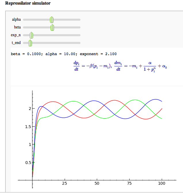
For a slightly more real-world example, suppose we want to interactively explore the behavior of a system of ODEs as we change parameters. The example below uses the "repressilator" system of Elowitz and Leibler [3], and a crude Euler's method (just for illustrative purposes!) to solve it. The behavior is not too bad for smaller runs but it gets a bit sluggish as we increase the simulation time.
def m_der(m,p,a,a0,n):
   return -m + a/(1+p^n) - a0
def p_der(m,p,b):
   return -b*(p-m)
def der_vec(m_list,p_list,a,a0,n,b):
   d_vec = []
   for i in (0,1,2):
       d_vec.append(m_der(m_list[i],p_list[(i+1)%3],a,a0,n))
   for i in (0,1,2):
       d_vec.append(p_der(m_list[i],p_list[i],b))
   return d_vec
def repressilator_run(m_init = [.1,.2,.3], p_init = [.1,.2,.3], a_val = 6, b_val = .1, n_val = 2.1, t_end = 100):
   a0_val = .01
   t_0 = 0
   stepsize = .1
   t = 0
   m_data = m_init,p_init,t
   while t < t_end:
       der = der_vec(m_data[-1][0],m_data[-1][1],a_val,a0_val,n_val,b_val)
       new_m = [m_data[-1][0][i] + stepsize*der[i] for i in (0,1,2)]
       new_p = [m_data[-1][1][i-3] + stepsize*der[i] for i in (3,4,5)]
       m_data.append([new_m,new_p,t])
       t = t + stepsize
   return m_data
bdigits = RealField(16)
print "Repressilator simulator"
@interact
def rep_run(alpha = slider(0,20,.01,10), beta = slider([10^i for i in srange(-3,1,.1)], default = .1), exp_n = slider(1,10,.1,2.1), t_end = slider([10^i for i in srange(0,3,.1)],default = 2)):
   test = repressilator_run(a_val = alpha, n_val = exp_n)
   html('beta = ' + str(bdigits(beta)) + '; alpha = ' + str(bdigits(alpha))+ '; exponent = ' + str(bdigits(exp_n)))
   print jsmath('\\frac{d p_{i}}{dt} = -\\beta (p_i - m_i), \ \\frac{d m_{i}}{dt} = -m_i + \\frac{\\alpha}{1 + p_i^{n}} + \\alpha_0')
   show(sum([list_plot([[x[2],x[1][i]] for x in test], hue = i/3.0, plotjoined=True) for i in (0,1,2)]), ymin = 0)
If we time a typical short run, it takes about .3 seconds. The moderately Cythonized form below takes about .02 seconds - noticeably snappier (all these timings are on the same machine).
%cython
cdef m_der(m,p,a,a0,n):
   return float(-m + a/(1+p**n) - a0)
cdef p_der(m,p,b):
   return float(-b*(p-m))
cdef der_vec(m_list,p_list,a,a0,n,b):
   d_vec = []
   for i in (0,1,2):
       d_vec.append(m_der(m_list[i],p_list[(i+1)%3],a,a0,n))
   for i in (0,1,2):
       d_vec.append(p_der(m_list[i],p_list[i],b))
   return d_vec
def repressilator_run(m_init = [.1,.2,.3], p_init = [.1,.2,.3], a_val = 6, b_val = .1, n_val = 2.1, t_end = 100):
   cdef float a0_val, t_0, stepsize, t
   a0_val = .01
   t_0 = 0
   stepsize = .1
   t = 0
   m_data = m_init,p_init,t
   while t < t_end:
       der = der_vec(m_data[-1][0],m_data[-1][1],a_val,a0_val,n_val,b_val)
       new_m = [m_data[-1][0][i] + stepsize*der[i] for i in (0,1,2)]
       new_p = [m_data[-1][1][i-3] + stepsize*der[i] for i in (3,4,5)]
       m_data.append([new_m,new_p,t])
       t = t + stepsize
   return m_data
Note that the above code is still using quite a few python objects and methods, and could be sped up further with more effort.
Other notes
Sage includes scipy, numpy, and matplotlib for 2D plotting. For 3D plotting, Sage has Jmol and the tachyon raytracer.
Sage is also notable for its friendly community. In particular, if you get stuck you can usually get very fast support by writing to the sage-support list. There is also pretty good documentation available.
There is much more to Sage but hopefully this introduction has whet your appetite.
References
-
"A Synthetic Oscillatory Network of Transcriptional Regulators"; Michael B. Elowitz and Stanislas Leibler; Nature. 2000 Jan 20;403(6767):335-8.


