Dahlquist:BioQUEST Summer Workshop 2015

Home        Research        Protocols        Notebook        People        Publications        Courses        Contact       

This is based on the most current version of the data analysis protocol for the Dahlquist Lab microarray data, which can be found on the Microarray Data Analysis Workflow page.

Summary of steps for microarray data analysis

1. Quantitate the fluorescence signal in each spot (GenePix Pro)
2. Calculate the ratio of red/green fluorescence (GenePix Pro)
3. Log transform the ratios (GenePix Pro)
4. Normalize the ratios on each microarray slide (within-chip normalization)
5. Normalize the ratios for a set of slides in an experiment (between-chip normalization)
6. Perform statistical analysis on the ratios
   • Within-strain ANOVA
   • Modified t test for each timepoint
   • Between-strain ANOVA
   • Benjamini & Hochberg and Bonferroni p value corrections for the above three tests
   • "Sanity Check" on above three tests
7. Pattern finding algorithms (clustering with stem)
8. Gene Ontology term enrichment analysis (on clusters with stem or on gene sets with MAPPFinder)
9. Pathway analysis (GenMAPP)
10. Determining candidate transcription factors and gene regulatory network (YEASTRACT)
11. Dynamical modeling with GRNmap; visualization with GRNsight

This page has instructions for steps 7,8, and 10.

Before you begin...

You will record all of the manipulations of the data in an electronic lab notebook stored on this wiki. Please see the Wiki Checklist page for more details on how to do this.

Viewing File Extensions

• The Windows 7 operating systems defaults to hiding file extensions. To turn them back on, do the following:

  

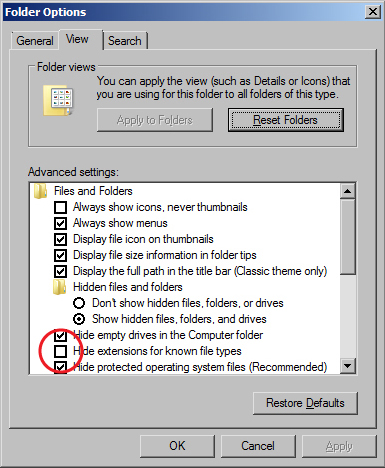
  Folder Options window

  1. Go to the Start menu and select "Control Panel".
  2. In the window that appears, search for "Folder Options" in the search field in the upper right hand corner.
  3. Click on "Folder Options" in the main window.
  4. When the Folder Options window appears, click on the View tab.
  5. Uncheck the box for "Hide extensions for known file types".
  6. Click the OK button.
• The computers in Seaver 120 are are set to erase all custom user settings and restore the defaults once they have been restarted, so you will probably have to do this many times throughout the semester when using these computers.

Set Your Browser to Prompt You for the Location to Save your Downloaded Files

• In Mozilla Firefox, open the Options window.
  • Select the radio button that says "Always ask me where to save files".
  • You could also change the default "Save files to" location to your Desktop, so that will be the first choice when it prompts you where to save the file. (You will have to temporarily deselect the radio button to do this and then reselect it when you are done.
  • Click OK to save your changes.
• In Google Chrome, open the Settings window.
  • Click on the link at the bottom of the page that says "Advanced Settings".
  • Check the box that says "Ask where to save each file before downloading".
  • You could also change the default Download location to your Desktop, so that will be the first choice when it prompts you where to save the file.
  • Your settings are automatically saved.

Step 7-8: Clustering and GO Term Enrichment with stem

1. Prepare your microarray data file for loading into STEM.
   • Here is a sample file formatted properly for stem: Dahlquist_dCIN5_data_for_STEM_BioQUEST2015.txt. Right-click on the link and choose "Save file as..." to save it to your computer (if you just left-click on it, most browsers will open it in the browser window instead of downloading it).
2. Now download and extract the STEM software. Click here to go to the STEM web site.
   • The full instructions for formatting your file can be found here.
   • Click on the download link, register, and download the stem.zip file to your Desktop.
   • Unzip the file. In Seaver 120, you can right click on the file icon and select the menu item 7-zip > Extract Here.
   • This will create a folder called stem. Inside the folder, double-click on the stem.jar to launch the STEM program.
3. Running STEM
   1. In section 1 (Expression Data Info) of the the main STEM interface window, click on the Browse... button to navigate to and select your file.
      • Click on the radio button No normalization/add 0.
      • Check the box next to Spot IDs included in the data file.
   2. In section 2 (Gene Info) of the main STEM interface window, select Saccharomyces cerevisiae (SGD), from the drop-down menu for Gene Annotation Source. Select No cross references, from the Cross Reference Source drop-down menu. Select No Gene Locations from the Gene Location Source drop-down menu.
   3. In section 3 (Options) of the main STEM interface window, make sure that the Clustering Method says "STEM Clustering Method" and do not change the defaults for Maximum Number of Model Profiles or Maximum Unit Change in Model Profiles between Time Points.
   4. In section 4 (Execute) click on the yellow Execute button to run STEM.
4. Viewing and Saving STEM Results
   1. A new window will open called "All STEM Profiles (1)". Each box corresponds to a model expression profile. Colored profiles have a statistically significant number of genes assigned; they are arranged in order from most to least significant p value. Profiles with the same color belong to the same cluster of profiles. The number in each box is simply an ID number for the profile.
      • Click on the button that says "Interface Options...". At the bottom of the Interface Options window that appears below where it says "X-axis scale should be:", click on the radio button that says "Based on real time". Then close the Interface Options window.
      • Take a screenshot of this window (on a PC, simultaneously press the Alt and PrintScreen buttons to save the view in the active window to the clipboard) and paste it into a PowerPoint presentation to save your figures.
   2. Click on each of the SIGNIFICANT profiles (the colored ones) to open a window showing a more detailed plot containing all of the genes in that profile.
      • Take a screenshot of each of the individual profile windows and save the images in your PowerPoint presentation.
      • At the bottom of each profile window, there are two yellow buttons "Profile Gene Table" and "Profile GO Table". For each of the profiles, click on the "Profile Gene Table" button to see the list of genes belonging to the profile. In the window that appears, click on the "Save Table" button and save the file to your desktop. Make your filename descriptive of the contents, e.g. "wt_profile#_genelist.txt", where you replace the number symbol with the actual profile number.
      • For each of the significant profiles, click on the "Profile GO Table" to see the list of Gene Ontology terms belonging to the profile. In the window that appears, click on the "Save Table" button and save the file to your desktop. Make your filename descriptive of the contents, e.g. "wt_profile#_GOlist.txt", where you use "wt", "dGLN3", etc. to indicate the dataset and where you replace the number symbol with the actual profile number. At this point you have saved all of the primary data from the STEM software and it's time to interpret the results!
5. Analyzing and Interpreting STEM Results
   1. Select one of the profiles you saved in the previous step for further intepretation of the data. I suggest that you choose one that has a pattern of up- or down-regulated genes at the early (first three) timepoints. You and your partner will choose the same profile so that you can compare your results between the two strains. Answer the following:
      • Why did you select this profile? In other words, why was it interesting to you?
      • How many genes belong to this profile?
      • How many genes were expected to belong to this profile?
      • What is the p value for the enrichment of genes in this profile? Bear in mind that we just finished computing p values to determine whether each individual gene had a significant change in gene expression at each time point. This p value determines whether the number of genes that show this particular expression profile across the time points is significantly more than expected.
      • Open the GO list file you saved for this profile in Excel. This list shows all of the Gene Ontology terms that are associated with genes that fit this profile. Select the third row and then choose from the menu Data > Filter > Autofilter. Filter on the "p-value" column to show only GO terms that have a p value of < 0.05. How many GO terms are associated with this profile at p < 0.05? The GO list also has a column called "Corrected p-value". This correction is needed because the software has performed thousands of significance tests. Filter on the "Corrected p-value" column to show only GO terms that have a corrected p value of < 0.05. How many GO terms are associated with this profile with a corrected p value < 0.05?
      • Select 10 Gene Ontology terms from your filtered list (either p < 0.05 or corrected p < 0.05).
        • Since you and your partner are going to compare the results from each strain for the same cluster, you can either:
          • Choose the same 10 terms that are in common between strains.
          • Choose 10 terms that are different between the strains (5 or so from each).
          • Choose some that are the same and some that are different.
        • Look up the definitions for each of the terms at http://geneontology.org. For your final lab report, you will discuss the biological interpretation of these GO terms. In other words, why does the cell react to cold shock by changing the expression of genes associated with these GO terms? Also, what does this have to do with HAP4 being deleted?
        • To easily look up the definitions, go to http://geneontology.org.
        • Copy and paste the GO ID (e.g. GO:0044848) into the search field at the upper left of the page called "Search GO Data".
        • In the results page, click on the button that says "Link to detailed information about <term>, in this case "biological phase"".
        • The definition will be on the next results page, e.g. here.

Step 10: YEASTRACT

Using YEASTRACT to Infer which Transcription Factors Regulate a Cluster of Genes

In the previous analysis using STEM, we found a number of gene expression profiles (aka clusters) which grouped genes based on similarity of gene expression changes over time. The implication is that these genes share the same expression pattern because they are regulated by the same (or the same set) of transcription factors. We will explore this using the YEASTRACT database.

1. Open the gene list in Excel for the one of the significant profiles from your stem analysis. Choose a cluster with a clear cold shock/recovery up/down or down/up pattern. You should also choose one of the largest clusters.
   • Copy the list of gene IDs onto your clipboard.
2. Launch a web browser and go to the YEASTRACT database.
   • On the left panel of the window, click on the link to Rank by TF.
   • Paste your list of genes from your cluster into the box labeled ORFs/Genes.
   • Check the box for Check for all TFs.
   • Accept the defaults for the Regulations Filter (Documented, DNA binding plus expression evidence)
   • Do not apply a filter for "Filter Documented Regulations by environmental condition".
   • Rank genes by TF using: The % of genes in the list and in YEASTRACT regulated by each TF.
   • Click the Search button.
3. Answer the following questions:
   • In the results window that appears, the p values colored green are considered "significant", the ones colored yellow are considered "borderline significant" and the ones colored pink are considered "not significant". How many transcription factors are green or "significant"?
   • List the "significant" transcription factors on your wiki page, along with the corresponding "% in user set", "% in YEASTRACT", and "p value".
     • Are CIN5, GLN3, HAP4, HMO1, SWI4, and ZAP1 on the list?
4. For the mathematical model that we will build, we need to define a gene regulatory network of transcription factors that regulate other transcription factors. We can use YEASTRACT to assist us with creating the network. We want to generate a network with approximately 15-30 transcription factors in it.
   • You need to select from this list of "significant" transcription factors, which ones you will use to run the model. You will use these transcription factors and add CIN5, GLN3, HAP4, HMO1, SWI4, and ZAP1 if they are not in your list. Explain in your electronic notebook how you decided on which transcription factors to include. Record the list and your justification in your electronic lab notebook.
   • Go back to the YEASTRACT database and follow the link to Generate Regulation Matrix.
   • Copy and paste the list of transcription factors you identified (plus CIN5, HAP4, GLN3, HMO1, SWI4, and ZAP1) into both the "Transcription factors" field and the "Target ORF/Genes" field.
   • In the context of a course, my students generate several regulation matrices, with different "Regulations Filter" options as described below. However, I know that the DNA-binding only evidence produces the appropriate density of network edges for modeling purposes.
     • For the first one, accept the defaults: "Documented", "DNA binding plus expression evidence"
     • Click the "Generate" button.
     • In the results window that appears, click on the link to the "Regulation matrix (Semicolon Separated Values (CSV) file)" that appears and save it to your Desktop. Rename this file with a meaningful name so that you can distinguish it from the other files you will generate.
     • Repeat these steps to generate a second regulation matrix, this time applying the Regulations Filter "Documented", "Only DNA binding evidence".
     • Repeat these steps a third time to generate a third regulation matrix, this time applying the Regulations Filter "Documented", DNA binding and expression evidence".

Visualizing Your Gene Regulatory Networks with GRNsight

We will analyze the regulatory matrix files you generated above in Microsoft Excel and visualize them using GRNsight to determine which one will be appropriate to pursue further in the modeling.

1. First we need to properly format the output files from YEASTRACT. You will repeat these steps for each of the three files you generated above.
   • Open the file in Excel. It will not open properly in Excel because a semicolon was used as the column delimiter instead of a comma. To fix this, Select the entire Column A. Then go to the "Data" tab and select "Text to columns". In the Wizard that appears, select "Delimited" and click "Next". In the next window, select "Semicolon", and click "Next". In the next window, leave the data format at "General", and click "Finish". This should now look like a table with the names of the transcription factors across the top and down the first column and all of the zeros and ones distributed throughout the rows and columns. This is called an "adjacency matrix." If there is a "1" in the cell, that means there is a connection between the trancription factor in that row with that column.
   • Save this file in Microsoft Excel workbook format (.xlsx).
   • Check to see that all of the transcription factors in the matrix are connected to at least one of the other transcription factors by making sure that there is at least one "1" in a row or column for that transcription factor. If a factor is not connected to any other factor, delete its row and column from the matrix. Make sure that you still have somewhere between 15 and 30 transcription factors in your network after this pruning.
     • Only delete the transcription factor if there are all zeros in its column AND all zeros in its row. You may find visualizing the matrix in GRNsight (below) can help you find these easily.
   • For this adjacency matrix to be usable in GRNmap (the modeling software) and GRNsight (the visualization software), we need to transpose the matrix. Insert a new worksheet into your Excel file and name it "network". Go back to the previous sheet and select the entire matrix and copy it. Go to you new worksheet and click on the A1 cell in the upper left. Select "Paste special" from the "Home" tab. In the window that appears, check the box for "Transpose". This will paste your data with the columns transposed to rows and vice versa. This is necessary because we want the transcription factors that are the "regulatORS" across the top and the "regulatEES" along the side.
   • The labels for the genes in the columns and rows need to match. Thus, delete the "p" from each of the gene names in the columns. Adjust the case of the labels to make them all upper case.
   • In cell A1, copy and paste the text "rows genes affected/cols genes controlling".
2. Now we will visualize what these gene regulatory networks look like with the GRNsight software.
   • Go to the GRNsight home page (you can either use the version on the home page or the beta version.
   • Select the menu item File > Open and select one of the regulation matrix .xlsx file that has the "network" worksheet in it that you formatted above. If the file has been formatted properly, GRNsight should automatically create a graph of your network. Move the nodes (genes) around until you get a layout that you like and take a screenshot of the results. Paste it into your PowerPoint presentation. Repeat with the other two regulation matrix files. You will want to arrange the genes in the same order for each screenshot so that the graphs can be easily compared.

Step 11: GRNmap

Running GRNmap from the Executable

1. Open Google Chrome or Firefox and navigate to the GRNmap home page by following this link. Click on the "Downloads" button located in the navigation bar at the left of the screen to go to the Downloads page.
2. You may have to disable the virus software on your computer because the GRNmap website may not be trusted on all computers.
3. Click "Download GRNmap Executables", find "GRNmap v1.0.10", and then click the green button that says "Download GRNmap_v1.0.10.zip executable" and save the file to the desktop. The computer settings may automatically save the file to the "Downloads" folder. If this is the case, drag the .zip file to the desktop.
4. An alternative method of downloading GRNmap is to go to the GRNmap GitHub site and follow the link. Select "Releases" and click "GRNmap_v1.0.10.zip". This method should work without changing the security settings of the anti-virus software.
5. Once "GRNmap_v1.0.10.zip" has been downloaded, extract the zipped file.
6. The extracted file should be named "GRNmap_v1.0.10". Open this folder, open the subfolder "GRNmap_v1.0.10", and double click the program called "MyAppInstaller_mcr.exe" When prompted select "Run". This may take a few minutes to install.
   • You will be prompted to an installer window, you must have administrator privileges to install the MATLAB compiler library. When the GRNmap Installer window appears, click "Next" to start the installation process. A dialogue box titled "Preparing Files" will appear with a status bar monitoring the process of the program "Assembling product list...". It will then ask you to designate a installation folder. Accept the default location C:\Program Files\GRNmap. It will warn you that this folder does not exist and ask if you would like to create it. Click "Yes" then press "Next." The next window asks where you would like the "MATLAB Compiler Runtime" installed. Accept the default location C:\Program Files\MATLAB\MATLAB Compiler Runtime. It will warn you that this folder does not exist and ask if you would like to create it. Click "Yes" then press "Next."
7. Accept the terms of the license agreement by selecting "Yes" and then pressing "Next." On the next screen press "Install" and a status bar will appear. Once the installation is complete, select "Finish".
8. Navigate to the "GRNmap_v.1.0.10" folder on the desktop and double click the program "GRNmap" and select "Run".
9. Two sample input workbooks are included with the executable package.
   • The input "4-genes_6-edges_artificial-data Sigmoidal_estimation_fixb-0_fixP-0_graph" will demonstrate all of the features of GRNmap and will run quickly. The file "22-genes_47-edges_Dahlquist-data_Sigmoidal_estimation_fixb-0_fixP-0_graph.xlsx" is more realistic, but will take up to 30 minutes to run.
10. GRNmap will open a dialogue box called "Select Input Worksheet for Simulation." Navigate to the directory that has your input file and select it.
11. A Matlab dialogue box called "Figure 1" should pop up on the screen. There should be two plots on the screen following the program's progress, and a counter number.
12. If you selected an input sheet with the option to make graphs, you will know the model has finished running when the program chimes (if your sound is on) and plots of the four difference genes appear on the screen. If you selected the option "no-graph" you will know the model has finished running when the counter number stops increasing. The counter image ("figure 1"), plots, output .xlsx file, and output .mat file should be save to the folder where the input sheet was saved. The plots and output sheets can be compared to the sample output included with the executable.
13. In order for the program to save the outputs successfully, none of the directories (folder name or user name) can have any spaces.

Follow this link for documentation for the input workbook format and the output workbook format.

Analyzing GRNmap Results

1. Create a new workbook for analyzing the weight data. In this workbook, create a new sheet: call it estimated_weights. In this new worksheet, create a column of labels of the form ControllerGeneA -> TargetGeneB, replacing these generic names with the standard gene names for each regulatory pair in your network. Remember that columns represent Controllers and rows represent Targets in your network and network_weights sheets.
2. Extract the non-zero optimized weights from their worksheet and put them in a single column next to the corresponding ControllerGeneA -> TargetGeneB label.
3. Now we will run the model a second time, this time estimating the threshold parameters, b. Save the input workbook that you previously created as a new file with a meaningful name (e.g. append "estimate-b" to the previous filename), and change fix_b to 0 in the "optimization_parameters" worksheet, so that the thresholds will be estimated. Rerun GRNmodel with the new input sheet.
4. Repeat Parts (4) through (6) with the new output.
5. Create an empty excel workbook, and copy both sets of weights into a worksheet.
6. Create a bar chart in order to compare the "fixed b" and "estimated b" weights.
7. Create bar charts to compare the production rates from each run.
8. Copy the two bar charts into your powerpoint.
9. Visualize the output of each of your model runs with GRNsight.
   • In order for this to work, you need to alter your output workbook slightly. You need to change the name of the sheet called "out_network_optimized_weights" to "network_optimized_weights"; i.e., delete the "out_" from that sheet name.
   • Arrange the genes in the same order you used to display them previously when you visualized the networks from YEASTRACT for both of your model output runs. Take a screenshot of each of the results and paste it into your PowerPoint presentation. Clearly label which screenshot belongs to which run.
   • Note that GRNsight will display differently now that you have estimated the weights. For positive weights > 0, the edge will be given a regular (pointy) arrowhead to indicate an activation relationship between the two nodes. For negative weights < 0, the edge will be given a blunt arrowhead (a line segment perpendicular to the edge direction) to indicate a repression relationship between the two nodes. The thickness of the edge will vary based on the magnitude of the absolute value of the weight. Larger magnitudes will have thicker edges and smaller magnitudes will have thinner edges. The way that GRNsight determines the edge thickness is as follows. GRNsight divides all weight values by the absolute value of the maximum weight in the matrix to normalize all the values to between zero and 1. GRNsight then adjusts the thickness of the lines to vary continuously from the minimum thickness (for normalized weights near zero) to maximum thickness (normalized weights of 1). The color of the edge also imparts information about the regulatory relationship. Edges with positive normalized weight values from 0.05 to 1 are colored magenta; edges with negative normalized weight values from -0.05 to -1 are colored cyan. Edges with normalized weight values between -0.05 and 0.05 are colored grey to emphasize that their normalized magnitude is near zero and that they have a weak influence on the target gene.
10. Interpret the results of the model simulation.
    • Examine the graphs that were output by each of the runs. Which genes in the model have the closest fit between the model data and actual data? Which genes have the worst fit between the model and actual data? Why do you think that is? (Hint: how many inputs do these genes have?) How does this help you to interpret the microarray data?
    • Which genes showed the largest dynamics over the timecourse? In other words, which genes had a log fold change that is different than zero at one or more timepoints. The p values from the Week 11 ANOVA analysis are informative here. Does this seem to have an effect on the goodness of fit (see question above)?
    • Which genes showed differences in dynamics between the wild type and the other strain your group is using? Does the model adequately capture these differences? Given the connections in your network (see the visualization in GRNsight), does this make sense? Why or why not?
    • Examine the bar charts comparing the weights and production rates between the two runs. Were there any major differences between the two runs? Why do you think that was? Given the connections in your network (see the visualization in GRNsight), does this make sense? Why or why not?
    • Finally, based on the results of your entire project, which transcription factors are most likely to regulate the cold shock response and why?
    • What future directions do you want to take?