Beauchamp:UsingTORTOISE

Beauchamp Lab

• Home
• Lab Notebook
• Publications
• People/Projects/Media
• Teaching
• Positions
• Data Sharing
• RAVE

Introduction This page describes using the program | TORTOISE to process DTI data. As may be surmised from the name (where T and O stand for "tolerably obsessive" and there's no need to remember the rest), the advantage of using TORTOISE is that there is considerable efforts put into QC-ing your DTI data, but the program is not particularly speedy. Downloading TORTOISE TORTOISE is distributed by NIH. The program can be downloaded from their website (https://science.nichd.nih.gov/confluence/display/nihpd/TORTOISE). Follow instructions there. Get your data You can use dcm2niix (Turning the raw data into AFNI BRIKs) to convert your data from dicoms. You should have 3 files for your DTI data- a .nii, .bval, and .bvec. These are the image data, the gradient strength (b-values) and the gradient direction vectors, respectively. At this point, I highly recommend moving the data to the shortest filename format you can manage. TORTOISE appends things to the filename as you go, so by the time you're finished you'll appreciate a short filename so you can see everything in the folder at once. TORTOISE keeps the three files (and other information, if you have it) together using a .list file. This is, as the name suggests, something like a list of the relevant files. To have TORTOISE generate one of these, use the ImportNIFTI command: data_path=/Volumes/data/<location_of_your_data> ImportNIFTI -i $data_path/*.nii -b $data_path/*.bval -v $data_path/*.bvec -p vertical These tell TORTOISE where the three files (.nii, .bval, .bvec) are, and indicate the phase encode direction, which in this case is vertical (that is, A-P on an axial acquisition). Vertical is the most common. When you run these, TORTOISE will create a new folder in $data_path with the suffix _proc. (the filename appending begins...) Inside that folder, you now have a .list file which points to your data. First Data Check At this point, we're going to run a quick'n'dirty tensor fitting, just to make sure everything looks about right. These are not data you would process. Instead, we're going to generate a glyph map of a single slice, just to make sure everything looks about right. 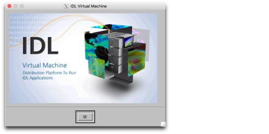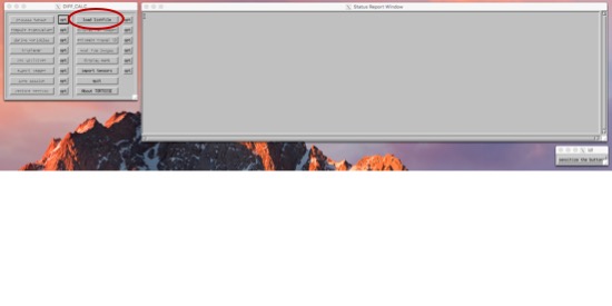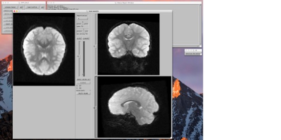EstimateTensorWLLS -i $data_path/*_proc/*.list ComputeGlyphMaps $data_path/*_proc/*L0_DT.nii open $data_path/*_proc/*.png This should only take a few minutes. When it's finished, you'll have a .png (image) file with a central slice of your data. On top will be a bunch of colored ovals, and these indicate the direction and anisotrophy of the tensors it would calculate. You should be able to see long ovals in the white matter, ovals that seem to follow each other, and ovals with colors that look like a color FA map. At this stage, it's most important to check that your gradients weren't rotated inappropriately (especially if you acquired your data obliquely). Prep the Structurals It's useful to have your data ACPC aligned. When you color-ize your FA map, it's useful if "anterior to posterior" in one subject is the same as the next subject. But, we don't want to stretch the data (as you would when you align to a template), just re-orient it. One way to do this is using the AFNI gui. If you have both a T1- and T2- weighted image for your subject, you can start by aligning these two scans together. align_epi_anat.py -anat t1_mprage.nii -epi t2_space.nii -epi_base 0 -epi_strip 3dSkullStrip -edge -epi2anat Then, you can use the AFNI gui to add markers to the T1, and apply these to your T2. Write these datasets out using the gui. Another (probably preferable) way to do this is to use fat_proc_axialize, detailed instructions here. Here, you can specify an atlas to compare your data to, and have it do only the translation/rotation parts of the warp. These two methods will do philosophically similar things, but mathematically a bit different. (Which is to say, don't try to check that one method or the other worked by viewing the results on top of each other.) Note - The fat_proc_axialize notes describe axializing the T2 and then aligning the T1 to the axialized T2. But this isn't your only choice. You could also axialize your T1 to a T1-weighted template, such as MNI152, TT_N27, or something more esoteric, like the Haskins pediatric atlas or a monkey atlas or whatnot. If you need a special atlas to match your data, this will probably dominate the decision to axialize the T1 and align the T2, or the other way around. If you are axializing a T1, the next recommended fatcat step (fat_proc_align_anat_pair) may not work so well. Instead, I'd try align_epi_anat.py. If you ultimately want to compare these DTI data to surface data, I would do this step *before* your freesurfer recon. It's not absolutely necessary (you can align your DTI data back to whatever surface you recon-ed), but it will make your life a bit easier. Just make sure you zero-pad your axialized T1 to a 1mm 256x256x256 grid on your own terms before you start, so they stay in register. Motion, Distortion Correction using DIFFPREP In order to run diffprep, you need to have a structural image. (To correct a distortion, it's useful to know what an un-distorted image looks like.) The TORTOISE gurus recommend a T2-weighted anatomical with fat suppression. That type of image will match contrast to the DWI images best, but will not have any distortion. In lieu of that, you could use a T1-weighted image, or (in a pinch) the motion-corrected average of all of your b=0 volumes. The axialize step (above) is optional, but useful. DIFFPREP -i $data_path/*_proc/*.list -s <path_to_structural_image> --will_be_drbuddied 0 --do_QC Now, grab a quick cup of coffee, and move on to something else for a bit. This will take a little while (maybe about an hour or two). If you have both a T1 and a T2, and you've added markers to the T1 so that it's AC-PC aligned (again, just rotated, not warped), then you could run this as... DIFFPREP -i $data_path/*_proc/*.list -s <path_to_T2> -r <path_to_ACPC_T1> --will_be_drbuddied 0 --do_QC Blip up blip down with DR_BUDDI If, as is becoming more and more recommended, you acquired half of your DTI data A-P and the other half P-A, then the next step would be to use DR_BUDDI. In that case, you'll want to do the above steps (import niftis, data check, diffprep) on each of them, and set --will_be_drbuddied to 1. All this does is tell DIFFPREP not to bother with the last few steps, because they'll be taken care of with DR_BUDDI. Then, after you run DIFFPREP, you'll run DR_BUDDI (which is also not a speedy program). The command for this is DR_BUDDI --up_data $data_path/*AP*proc/*_proc.list --down_data $data_path/*PA*proc/*_proc.list --structural <path_to_structural_image> If you're using connectome data (and this probably goes for many other multi-band sequences, as they tend to have long TEs), you may want to throw in a --distortion_level large flag as well, so it knows to allow for the larger distortions. Check your QC You should now have a folder called QC in $data_path/*_proc. This folder contains a series of useful images showing your data before and after the motion/distortion corrections. Calculate Tensors Now, we'll move into the TORTOISE GUI. This is run using an IDL virtual machine. In future versions, more and more functions will be moved to command line, but right now (version 3.1.1), we've run out of things we can do outside the IDL. In addition to moving to the IDL, you need to convert your data at this point from the new .list format to the old .list format. To do that, use this command: ConvertNewListfileToOld $data_path/*_proc/*_DMC.list Then, you can fire up the IDL cd /Applications/TORTOISE/DIFFCALC/DIFFCALCV25/DIFFCALC/diffcalc_main/ ./calcvm You'll see the splash screen, just hit ok. Now, three windows will pop up. I know, I know, you're wondering what that "sensitize the buttons" thing is. It's ok. You can push it if you want. The buttons on the main menu with be greyed out when you can't do things, and will become black when the function is available. BUT, if you close a window, or if there's some error, everything may get greyed out. At that point, you can "sensitize" the buttons again, and go back on your merry way. Import your listfile in OF. Sometimes, I find it easiest to sort these in the terminal window (ls -ltr) and just to be sure I'm getting the right one. Navigate to this listfile in the menu. From here, you're more or less going to move right down the list of things to do. You can... Look at the images, and if need be, remove volumes that have artifacts (e.g. due to motion). Estimate the noise in the image, and make/display a mask. one weird thing: when I "mask raw images," it takes a short while before the dialogue box says "Finished masking." and then "Processing mask ..." after it says "Processing mask ..." The Activity monitor shows CPU usage increase for a bit, then go back to zero, and as far as I can tell, it's done. BUT IT'S NOT. Something keeps happening. I know (ok, I think) this because, if I immediately ask it to display the mask, it won't, and a bunch of errors appear in the terminal where I ran calcvm. But, if I wait 10-15 minutes and come back, then it will display the mask. I'm not sure what this is about. .... just, let the mask cool down to room temp before you use it. 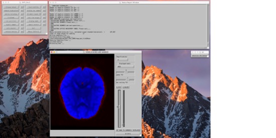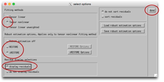Then you can process the tensor. First, click the box labeled "opt" next to "process tensor." We're going to use either the "RESTORE" or "iRESTORE" algorithm to process the tensors. iRESTORE is "informed" RESTORE, and takes into account additional information about the tissue types. This is under "Tensor nonlinear," so select that first, then choose (i)RESTORE (and choose options for this if you so desire). Finally, "display residuals" and "done." You should see a window pop up showing the residuals, and the program will run for a bit. When it's done, the dialogue box will say "DONE SAVING VARIABLES." Now, you can move down the left column of operations. You can Compute Eigenvalues, and derive variables (like FA). Tractography, if you so desire Now that you have your tensors fit, you can move on to doing other things with them. TORTOISE has an export tool, so you can export the tensor fitting and move on to other programs. TRACKVIS In the TORTOISE gui, export images as "PROCESSED FOR TRACKVIS." It will create a new folder within your current _proc directory, with the new files. Now, open Diffusion Toolkit. Turn on "Reconstruction." We're not actually going to reconstruct (you just did, with TORTOISE), but we'll use this to specify the files. Use the button next to the "Raw data files" filename to navigate to your new TORTOISE-ized _tensor file. When you do this, it will set the "Recon prefix" etc under Tracking. Un-check Reconstruction. Under Tracking, find the filename for "Recon prefix." You want this to be set such that, if you added '_tensor.nii' to the end of it, it would get to the file you just got from TORTOISE. In the data I have right now, that means that I need to replace "dti" in that field with "AP_proc_DRBUDDI_final_OF_R1". Once you change that, the "Save track as" and "Mask image" fields will change as well. Set "Mask Threshold," "Angle threshold," and any other settings you'd like to modify as you normally would. See here for more info. Now, hit "Run" and in a few minutes, you should have a beauteous hairy brain. :-)