BME100 f2013:W900 Group16 L5

BME 100 Fall 2013	Home People Lab Write-Up 1 | Lab Write-Up 2 | Lab Write-Up 3 Lab Write-Up 4 | Lab Write-Up 5 | Lab Write-Up 6 Course Logistics For Instructors Photos Wiki Editing Help
OUR TEAM Error creating thumbnail: File missing Laura Stanovich Error creating thumbnail: File missing Aakriti Gupta Error creating thumbnail: File missing Meilin Ossanna Error creating thumbnail: File missing Paul Lim Error creating thumbnail: File missing Kevin Liao LAB 5 WRITE-UP Background Information SYBR Green Dye SYBR green dye is a molecular dye that fluoresces in the presence of double stranded DNA, but fluoresces weaker in the presence of single stranded DNA. The dye stains the dsDNA produced through polymerase chain reaction (PCR). Single-Drop Fluorimeter The single-drop fluorimeter device detects and measures fluorescence by identifying and quantifying specific fluorescent molecules in a medium. The quantity of fluorescence is directly related to the amount of fluorescent material as well as the amount of molecule that is being detected. Below is an image of the single-drop fluorimeter device. Error creating thumbnail: File missing How the Fluorescence Technique Works A droplet of the material is placed on the superhyrophobic slide and is exposed to two light beams that decrease the surrounding noise. The fluorescent molecules generate light through excitation by shining light of a shorter wavelength. The energy is released in the form of a photon; the amount released will determine the photon's wavelength and the color of fluorescence which is specific to the SYBR green dye. Procedure Smart Phone Camera Settings We used an application for the camera and the timer on the iPhone and all of the settings were auto. 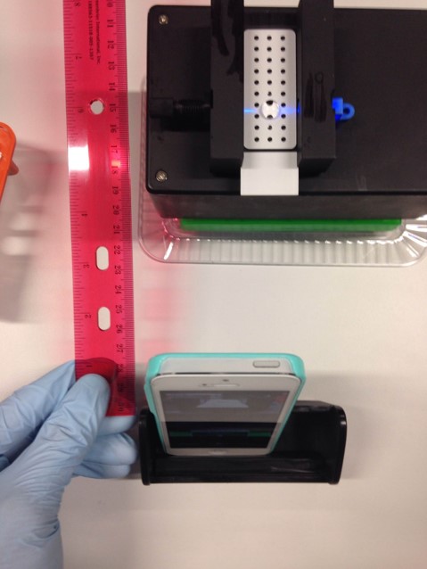Calibration Distance between the smart phone cradle and drop = 10 cm Distance between the smart phone camera to drop = 9 cm [Instructions: See worksheet page 6.] The picture above shows the distance at which the smart phone was placed from the fluorimeter. 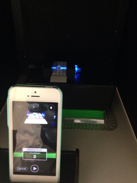The image above shows the entire setup under the black box while the samples were being photographed. Calf Thymus DNA Solution concentration (µg/mL) Volume of the 2X DNA solution (µL) Volume of the SYBR Green Final DNA concentration in SYBR Green I Assay (ng/mL) 5 80 80 2.5 2 80 80 1 1 80 80 0.5 0.5 80 80 0.25 0.25 80 80 0.125 0 80 80 blank Placing Samples onto the Fluorimeter To be ensure the samples placed on the slide would result in the correct calibration, the fluorimeter had to be set up properly. The slide was placed onto the fluorimeter and adjusted so that the line of blue light fell directly in between the first two rows of dots. After setting up the fluorimeter, the micro-pipetter was calibrated to 80 microliters and then attached to a clean tip. The tip was inserted into the SYBR Green microtube and then transferred to the slide in between the first two dots so that the blue light illuminated the drop. The contaminated tip was then thrown away. Using a fresh tip still at 80 microliters, the 0 concentration calf thymus was transferred to the slide on top of the already existing SYBR Green drop. The tip contaminated with calf thymus was also thrown away. After aligning the camera on the same plane as the slide and the blue light was directly in line with the drop, a black box was put over the fluorimeter and camera to ensure the blue light was the only light source. The micropipetter then transferred the drop on the slide into the red Dixie cup for proper waste disposal. This process was repeated five times with 0.25, 0.5, 1, 2, and 5 concentrations respectively. Each time, however, the positioning of the drops changed each time, using the next pair of dots with the blue light instead of just sticking with the first two rows the whole time. 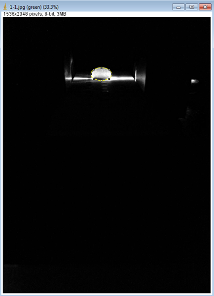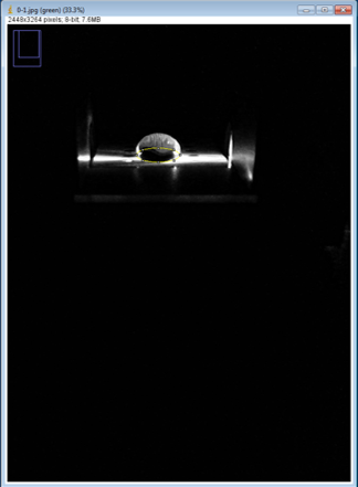Data Analysis Representative Images of Samples This is an image where a circle was drawn around the droplet with the freehand tool for a sample with no DNA This is an image where a circle was drawn around the droplet with the freehand tool for a sample with DNA Image J Values for All Samples Calf Thymus DNA Concentration (FINAL), ìg/mL ' AREA Mean Pixel Value Standard Deviation Of Drop RAWINTDEN - BACKGROUND Subtracted drop & Background 5 image 1 4748 237.792 33.446 1129037 10461 1118576 5 image 2 4154 242.575 28.777 1007657 9035 998622 5 image 3 4868 236.993 37.511 1153682 11881 1141801 2 image 1 11985 205.929 67.102 2468057 18891 2449166 2 image 2 13688 197.781 68.269 2707229 21565 2685664 2 image 3 12756 199.634 67.639 2546535 19279 2527256 1 image 1 5265 176.592 67.582 929758 5882 923876 1 image 2 3852 128.091 66.473 493406 5122 488284 1 image 3 5778 214.353 48.057 1238529 6692 1231837 0.5 image 1 13329 108.699 58.687 1448846 18442 1430404 0.5 image 2 13674 121.774 52.412 1665140 15932 1649208 0.5 image 3 12059 119.689 52.823 1443330 22226 1421104 0.25 image 1 4816 52.223 63.274 251508 5646 245862 0.25 image 2 5052 32.584 49.664 164615 6841 157774 0.25 image 3 5336 39.38 58.745 210133 6694 203439 0 image 1 13845 52.334 71.433 724565 14662 709903 0 image 2 11992 66.351 75.566 795687 12082 783605 0 image 3 13088 44.895 62.211 587588 23493 564095 Fitting a Straight Line 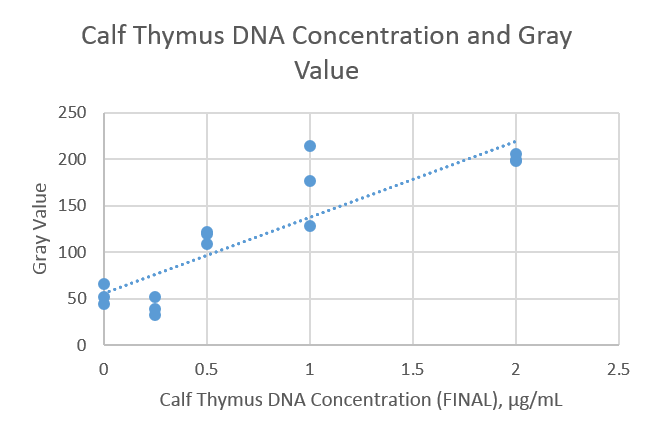The graph above shows the DNA concentration of the drops for every data point. There were three different data points per concentration. 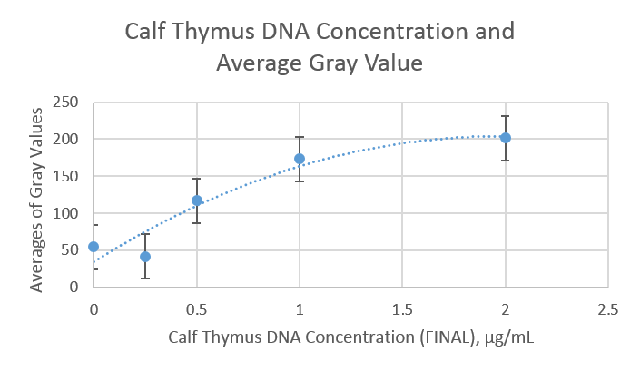As we were analyzing our data, we found out that our pictures were not calibrated correctly. Therefore, we decided to calibrate all of the data by hand on our graph. Once we had our data values such as the standard deviation, we multiplied the standard deviation by 2 because we wanted to find our error bar range. The averages and the error bars are shown in the graph above.