BE.180:Devices
Summary
The material on this page covers three topics. First, we briefly review how to make different sorts of gene-expression based devices. Second, we develop a simple framework for modeling the behavior of genetic devices. Third, we use the models to estimate some physical characteristics of our devices (for example, device latency).
Introduction
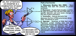
From before, you know that a genetically encoded inverter (i.e., a Boolean NOT gate) can be made by combining a ribosome binding site (RBS), driving expression of an open reading frame (ORF) encoding a repressor protein, followed by a transcription terminator. The signal is inverted when the repressor protein binds an operator site elsewhere on the DNA, resulting in repression of gene expression from the operator site. Click on Figures 1 and 2 below for more information (revisit the full comic if you need more background information for how genetically encoded inverters work).

Genetic Devices
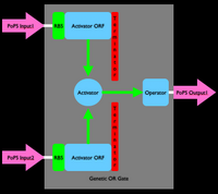
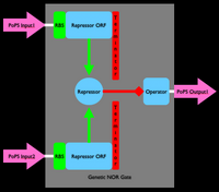
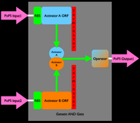
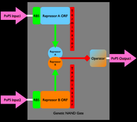
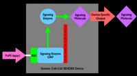
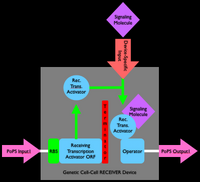
An inverter is one type of device. We can produce many different types of gene-expression based devices. For example, all sorts of logic gates can be implemented as gene-expression devices. We can also implement other sorts of devices such as sensors, actuators, and even cell-cell communication devices. Simple sketches and explanations of different gene-expression devices are given below. You can make many more types of genetic devices. The important concept to remember is that you want to make devices that allow subsequent hiding of the details for how the device actually works, so that other people can easily use your devices!
Device Modeling
The above depictions of genetic devices provide qualitative descriptions of device function (for example, if the input signal to an inverter is HIGH then the output signal from the inverter will be LOW). But, in reality, each device is a physical object, which imposes constraints on its exact operation and use. Here, we will use some simple modeling to get a sense for the physical behavior of our genetic devices. To start, let's define some of the device characteristics that we might care about. We'll use an inverter device as an example. One important property of our inverter is its transfer function, which is the steady state relationship between the device input and output signals. A second property is the device latency, which is the time it takes the device output signal to change in response to a change in the device input signal. To begin to model the inverter device we'll need to revisit the physical processes that are required for device operation. Our goal will be to build a model from these details that can be used to make some simple mathematical estimates of the inverter's transfer function and latency.
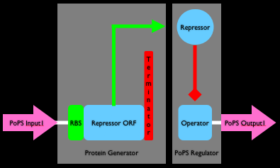
To make our analysis simpler let's split (decouple) an inverter into two sub-devices (Figure 4). The first sub-device is a "protein generator" (a protein generator takes a generic PoPS input signal and produces a specific protein as output). The second sub-device is a "PoPS regulator" (a PoPS regulator takes a specific regulatory protein as input and produces a generic PoPS signal as output). We'll model the transfer function and latency of each device individually and then combine the results in order to produce an overall model for our inverter.
Protein Generator Modeling
We need to develop a model that lets us estimate the transfer function (input:output relationship) and latency of the protein generator. The input to the protein generator is a PoPS input signal (let's call this P_in). The output is the concentration of the repressor protein (let's call this R). The transfer function should describe R as a function of P_in.
We can get started by writing down the physical processes that take place between arrival of a RNA polymerase molecule and the production of a repressor protein. First, the RNA polymerase enters the device and carries out transcription, producing a messenger RNA (mRNA) molecule. The RNA polymerase molecules will move basepair-by-basepair down the DNA encoding our protein generator device until they arrive at the terminator part (at which point they will stop transcription). Then, ribosomes will bind the newly produced mRNA molecules at the ribosome binding site (RBS) and start the process of protein synthesis (translation). The ribosomes will move nucleotide-by-nucleotide down the mRNA molecule until they arrive at a stop codon (in bacteria the triplets UAA, UGA & UAG can act as stop codons). To complete our model we should also account for the loss of mRNA and protein via mRNA and protein degradation, respectively. Furthermore, if the cell in which our device is operating is itself growing, then we may also need to account for the dilution of mRNA and protein levels via cell division. Phew! This is a lot of stuff to remember and pay attention to. How are we going to estimate transfer function and latency? Let's make a big simplification by writing down a differential equation that describes how the concentration of R changes over time:
We've introduced two new variables, [math]\displaystyle{ f(P_{in}) }[/math] and [math]\displaystyle{ k_d }[/math]. Here, [math]\displaystyle{ f(P_{in}) }[/math] is a placeholder function that describes the relationship between P_in, the PoPS input signal, and the rate of repressor protein synthesis. [math]\displaystyle{ k_d }[/math] is just a first-order decay rate for the loss of R. The first term in this equation makes a big leap directly from PoPS to protein synthesis (we're hiding all the details of transcription and translation). The second term in this equation captures the rate of destruction of R due to degradation (and dilution due to growth, if we want to include that too). If we can come up with some values for these terms in then we can estimate how R will change as a function of P_in and how quickly these changes will happen.
Let's start with [math]\displaystyle{ k_d }[/math]. [math]\displaystyle{ k_d }[/math] is the rate constant for protein degradation. The exact value of [math]\displaystyle{ k_d }[/math] will depend on the particular protein used in our device. Some proteins are incredibly stable and for all practical purposes don't degrade (for example, green fluorescent protein). Other proteins are actively degraded by the cell and will disappear quickly if they are not continuously being synthesized. Protein stability is typically reported in terms of a "half-life" (half-life, [math]\displaystyle{ t_{1/2} }[/math], is the amount of time it takes for one half of something, repressor protein in this case, to be degraded). So, a stable protein will have [math]\displaystyle{ t_{1/2} \approx \infty }[/math] whereas an unstable protein will have [math]\displaystyle{ t_{1/2} \approx 10 }[/math]minutes. You can quickly convert between a [math]\displaystyle{ t_{1/2} }[/math] and first-order [math]\displaystyle{ k_d }[/math] value via the following formula: [math]\displaystyle{ k_d = 0.69 / t_{1/2} }[/math]. Click here if you don't know where this formula comes from.
Without going through all the details, the value for [math]\displaystyle{ f(P_{in}) }[/math] might range from 0 to 100 proteins per minute (for a device that is present at single "copy number" per cell; copy number is the number of DNA molecules inside the cell carrying a particular gene, part, device or system). For this first example, let's use [math]\displaystyle{ t_{1/2} = 10 }[/math] minutes and an input range of [math]\displaystyle{ f(P_{in}) = }[/math] 0 to 70 proteins per minute. From [math]\displaystyle{ t_{1/2} = 10 }[/math] minutes we get [math]\displaystyle{ k_d \approx 0.07 }[/math] per minute. We can solve for the low and high steady state values of R by using the above equation. For example, at the low input value we get:
This shouldn't be surprising. Since we are not producing any R the steady state value of R is zero.
Next, at the high input value we get:
Thus, we now know the low and high range of the output signal R from our protein generator device. Furthermore, by setting the left side of equation 1 (above) to zero, we can provide a general formula for the steady-state output level of R as a function of P_in (Figure 5):
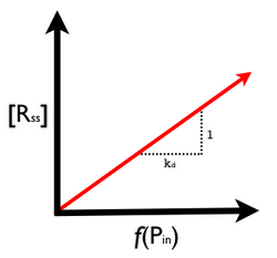
The next (last) thing to estimate using our model is the latency of the protein generator device. Again, latency is defined as the time it takes for the output signal of a device to reach a new level in response to a change in the input signal level. Because gene expression is a slow process (when compared, for example, to silicon-based computers) we'll need to pay close attention to issues of latency. Figure 6 below details the two types of latency we are interested in, low->high and high->low.
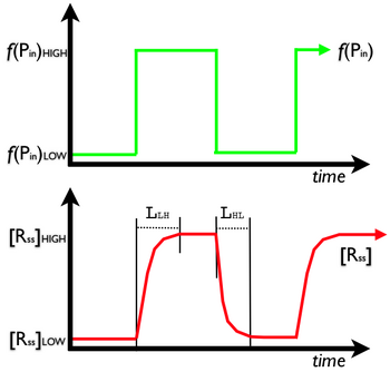
To estimate the latency during a LOW-to-HIGH transition ([math]\displaystyle{ L_{LH} }[/math]) we can again return to Equation 1 above. Imagine that there is no R present in the cell. How long does it take for the R level to reach its steady state concentration [math]\displaystyle{ [R_ss]=1000 }[/math] in response to a change in P_in from 0 to 70? One rough estimate is 1000/70 or ~14 minutes. However, this will be an underestimate because as the R level increases the newly produced R molecules will be subject to degradation. For now, we'll simply increase our [math]\displaystyle{ L_{LH} }[/math] estimate to ~20 minutes. To estimate the latency during a HIGH-to-LOW transition ([math]\displaystyle{ L_{HL} }[/math]) start by imagining a cell in which there are 1000 R molecules when, suddenly, the value of P_in drops from 70 to 0. How long will it take the level of R to drop to zero? From above we know that the level of R will drop by a factor of two every 10 minutes. For example, in 20 minutes the R level will drop to ~250 molecules per cell.
Thus, we've already been able to make a simple model and use it to estimate the transfer function and latency of our protein generator:
f(P_in) ranges from 0 to 70 proteins per minute.
R ranges from 0 to 1000 proteins per cell.
The full relationship between input and output can be expressed via Equation 2 (above).
It takes ~20 minutes for the output signal to respond to an increase in the input signal from 0 to 70 proteins per minute.
It also takes ~20 minutes for the output signal to respond to a decrease in the output signal from 70 to 0.
PoPS Regulator Modeling
Next, let's develop a model that we can use to estimate the transfer function and latency of the right half of our inverter, the "PoPS regulator." The input to the PoPS regulator is the concentratration of repressor protein, R. The output is a standard PoPS signal (let's call this P_out). Again, we'll get started by writing down the physical processes that take place during device operation.
First, R protein binds and interacts with an operator site on the DNA. Binding of the repressor protein to the operator site physically blocks (occludes) binding by RNA polymerase. When R is bound to the operator, no RNA polymerase can bind, so that the P_out signal is zero. When R is absent from the system RNA polymerase can bind the operator and initiation transcription, creating a high P_out signal.
The interaction between the R protein and the operator site can be modeled as a generic second order binding system, A+B<->AB (note that this is the same framework used to represent a simple ligand:receptor binding system); click here for a refresher. Using such a model, we'll want to estimate the fraction of operator site that is occupied by R protein at any instant in time. Let's start by using a simple differential equation that tracks the amount of repressor:DNA complex, R:D as a function of time:
Let's estimate some typical values for our rate constants. [math]\displaystyle{ k_on }[/math] is the rate at which R bind the operator site on DNA. Let's estimate that this is near the "diffusion limit" for proteins inside cells or 1E9/M*second. Next, let's consider what happens for a R:D complex that has a dissociation constant of 1nM ([math]\displaystyle{ K_D = 1E-9M }[/math]). From here we know that [math]\displaystyle{ K_D = k_{off}/k_{on} }[/math]. From this we can compute that [math]\displaystyle{ k_{off} }[/math] for our system is 1/second. We're almost ready to substitute these values into the above equation, but first we need to estimate one more thing, the concentration of DNA inside the cell. Bacteria usually a single copy of their genome inside the cell (fast growing bacteria and radiation resistant bacteria sometimes have multiple copies of their genomes). The volume of E.coli is approx. 1E-15L (it's a pretty small critter). Note that 1 moleculeper 1E-15L is the same concentration as 1E15 molecules per liter, which is about 1E-9M. Or, in other words, 1 molecule per E.coli cell is a concentration of ~1nM. Phew. Now we can start substituting into the above equation.
Which simplifies to:
From this equation alone we can get a sense for what the latency of our PoPS regulator will look like. Imagine that the input concentration of R goes instantly from 0 to 1000 proteins per cell. It will only take a couple seconds for the P_out signal to update. Similarly, if the R level drops from 1000 to 0, it should take a couple seconds for the P_out signal to rise. Thus, the latency of our PoPS regulator should be neglible compared to the tens of minutes required for our protein generator to respond.
What about a transfer function for the PoPS regulator? Like before, we need a function that will let us estimate P_out as a function of the input R concentration. To start, we know that at a zero R input level the P_out level will be maximum. We also know that at an infinite R input level that the P_out level should be zero. For the in between regions, if we can estimate the fraction of time that the operator site is bound by R then we can scale the maximum P_out level to reflect the actual P_out level as a function of R. Let's revisit some simple models. First, repressor and DNA form a complex with dissociation constant [math]\displaystyle{ K_D }[/math]:
Next, the repressor conservation of mass equation is:
Substitution gets us:
Solving for [R:D] produces:
Substituting into the conservation of mass equation (above) and dividing by [D_total] gets us the fraction of operator bound by R:
One minus this value is the fraction of operator unoccupied by R:
Phew! So, our P_out as a function of R looks like:
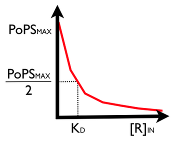
We won't go derive it here but note that you can tune the shape of the PoPS regulator's transfer function by using an activator in place of a repressor, or by using a repressor/activator molecule that binds as a dimer, tetramer or even a higher-order molecular complex. Many natural biological systems use dimeric and tetrameric DNA regulatory molecules to "sharpen" their dose-response transfer functions. This is useful for producing a "switch-like" dose response. For example, here's the generic form of the transer function for a repressor protein that binds as a N-mer (where N is the number of molecules required to bind the operator site on the DNA):
What sort of transfer function is produced for N=4?
Combining Models
OK. Now we can combine our two sub-device models to produce an estimate for overall device latency and input/output transfer function. Note that latency will be dominated by that of our protein generator sub-device. So, the device latency is still on a timescale of 10s of minutes. What about the transfer function? We want to go from PoPS_in to PoPS_out. Can we somehow combine the two sub-device transfer functions?
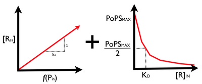
The short answer is YES but what happens and whether or not the resulting behavior is useful to us will depend on how the exact (that is, quantitative) signal levels match between our two devices. For example, is the R_out level from the protein generator device is much lower than the K_D value in our PoPS regulator device, no amount of response from the protein generator device will drive a response in the PoPS regulator. Ideally, we might want to start by designing our two sub-devices so that the middle R_out level from the protein generator is roughly equal to the K_D of the PoPS regulator. This will result in signal level matching between the two devices.
Combining the two steady state transfer functions from our subdevices produces an overall transfer function for our inverter device: