20.109(S13):Characterize protein expression (Day7)

Introduction

Today you will obtain titration curves against calcium for your wild-type and mutant proteins using an automated fluorescence plate reader. This machine reads multiple samples in a standard format – in our case, a 96-well microtiter plate. The output is a grid of up to 96 fluorescence values, for rows A-G and columns 1-12, which is amenable to analysis with a program like Excel.

In order to further benefit from this high-throughput testing format, you will make friends with the multichannel pipet, a purely mechanical rather than digital aid for repetitive experiments. This tool allows you to suck up and expel equivalent volumes of multiple identical samples (usually 8-12 at a time) with just one stroke. You will use this type of pipet to fill each row of a microtiter plate with one type of protein sample, and each column with a different concentration of calcium. Although a multichannel pipet can be sufficient for a typical research lab, in pharmaceutical companies that may be assaying thousands of samples a day, yet more steps of automation and scaling up are required, such as robotic pipet arms that obviate the need for manual pipetting at all. The degree of automation commercially available, or developed ‘in-house’ in a certain lab or corporation, depends in part on the frequency with which a certain assay is used. Assays used by many different labs and companies (such as fluorescence or absorbance spectrophotometry) are likely to breed commercially available high-throughput machines.

Error creating thumbnail: Unable to save thumbnail to destination

Signal:noise in arbitrary data collection. Background measurements (open circles), sample measurements (closed circles), and average values (short horizontal lines) are shown. The short line without any data points represents the reduction in average signal when background is subtracted. All measurements are with respect to an arbitrary vertical axis; the long horizontal line represents a measurement of zero.

While the concept of scale is a pragmatic concern, a perhaps more substantive topic of interest to us today is that of confidence in our results. As you are probably well-aware, every manipulation and measurement you make in the lab has an error associated with it. For example, consider the ubiquitous P200 pipetman. According to one pipet manufacturer, its accuracy is 1% (slightly worse at the lowest volumes). So an attempt to pipet 100 μL would result in an actual volume of 99-101 μL from the error of the instrument alone, which could be further compounded by a sleepy pipet operator, say. The precision of a pipet is typically better than its accuracy, 0.25% for the example given above. Precision refers to the reproducibility of a given measurement, not its absolute accuracy. This simple example demonstrates the general principles applicable to other types of error.

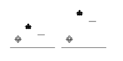
You will attempt to get a sense of the overall error of today’s experiment by running your protein samples in duplicate. That is, for each protein-calcium combination, you will perform two independent measurements. These measurements can then be averaged to smooth out your data, and hopefully improve the signal to noise ratio - where signal here refers to true differences between samples mixed with different amounts of calcium, and noise means inherent fluctuations in the system due to error. Noise in this experiment can also refer to background fluorescence of the sample buffer. Thus, another way to maintain a reasonable signal:noise ratio is by keeping our protein fairly concentrated, so that the absolute fluorescence values we obtain are high compared to the background. The figure at right demonstrates the above concepts. Scatter in the data (not all of the circles are at the same height) is one kind of noise. The level of background is another kind of noise: the left-hand data has a relatively low signal and thus poor signal:noise ratio, while the right-hand data has a relatively high absolute signal and improved signal:noise ratio.

Regarding the assay itself, note that we are using specially paired buffers to keep the concentration of calcium constant inside a given well. Otherwise, at low concentrations, as calcium began to bind to IPC it would be lost from the solution, thus distorting our measurement of binding and ultimately K_D.

Protocols

Everyone will begin with Part 1, due to its lengthy incubation steps. After that, about two groups at a time will work on Part 2. While you wait for your turn, feel free to work on the FNT, which is a high-level outline of your methods section.

Part 1: SDS-PAGE

1. Last time you prepared cell-normalized -IPTG and +IPTG samples and added Laemmli sample buffer (containing SDS, etc.) to them. Now you will complete protein denaturing in preparation for PAGE, alongside two different MW ladders.
   • The pre-stained ladder will be used to track gel progress.
   • The unstained ladder contains a known amount of protein per band and thus can be used to estimate gross protein contents.
2. Boil all 7 eppendorfs (including 15 μL of ladder!) for 5 minutes in the water bath that is in the fume hood.
3. You will be shown by the teaching faculty how to load your samples into the gel. You should load your samples according to the table below, one team per gel.
4. Note the starting and stopping time of electrophoresis, which will be initiated by the teaching faculty at 200 V, and run for 30-45 minutes.
5. Pry apart the plates using a spatula, and carefully transfer your gel to a staining box.
6. Add enough distilled water to cover the gel (say, 200 mL) and rinse the gel for 5 min on the shaker in the hood.
7. Repeat the rinse two more times with fresh water (~200 mL and 5 min incubation each time).
8. Add ~ 50 mL of BioSafe Coomassie, and incubate for at least 1 hour.
9. Empty the staining solution into the waste container in the fume hood - careful not to lose your gel!
10. Add 200 mL of water to your stained gel. Replace with fresh water just before leaving the lab if you have a chance.
11. Tomorrow, the teaching staff will transfer each gel to fresh water, then photograph them and post the results to the Day 7 Talk page.

Loading order and volumes

Loading volume is 10 μL for the ladder and 25 μL for your samples.

You may load your samples as -, -, -, +, +, + OR -, +, -, +, - +. Either way, please use the order WT, reference mutant, unique mutant.

It's best to load lanes 2-9 rather than 1-8, because the edge lanes on an SDS-PAGE often appear somewhat distorted.

Lane #	Sample Name	Lane #	Sample Name
2	pre-stained ladder	6	sample 4
3	sample 1	7	sample 5
4	sample 2	8	sample 6
5	sample 3	9	unstained ladder

Part 2: Prepare samples for titration curve

Tips for Success

Take great care today to limit the introduction of bubbles in your samples. When expelling fluid, pipet slowly while touching the pipet tip against the bottom or side of the well.

When using the multichannel pipet, always check to make sure all tips are getting filled - sometimes one tip may not be on all the way, and will pull up less volume than the others. If this happens, release the fluid, adjust the tip, and try again.

Protocol

Error creating thumbnail: Unable to save thumbnail to destination

Titration sample preparation

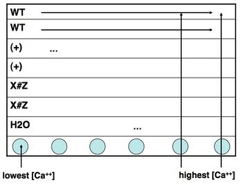
1. Take a black 96-well plate, and familiarize yourself with the scheme at right: top two rows are wild-type, next two rows are one of the reference mutants, and the final two sample rows are your own mutant. These are followed by a single blank/background row and an empty row.
   • The dark sides of the plate reduce "cross-talk" (i.e., light leakage) between samples in adjacent wells, another potential contribution to error.
2. Transfer an aliquot of wild-type protein to a plastic reservoir. Use the multichannel pipet to add 30 μL of protein (per well) to the top two rows of your plate.
   • Based on your protein volume, you should add about 4 wells at a time, and at the end may need to reduce down to 2 wells or even single additions.
3. Take a fresh reservoir or use the next compartment in a divided reservoir, and repeat step 2 for your mutant proteins, adding each one to the appropriately labeled rows.
4. Finally, add plain water with only BSA (no IPC) to the seventh row of the plate, using the shared dedicated reservoir. (Why do you think we are including this row of solutions?)
5. Using shared reservoir #1 (lowest calcium concentration), add 30 μL to the top seven rows in the first column of the plate. Discard the pipet tips.
6. Now work your way from reservoirs #2 to #12 (highest calcium concentration), and from the left-hand to the right-hand columns on your plate. Be sure to use fresh pipet tips each time! If you do contaminate a solution, let the teaching faculty know so they can put out some fresh solution. Honesty about a mistake is far preferred here to affecting every downstream experiment.
7. Finally, cover the plate with parafilm and wrap it in aluminum foil.

Part 3: Fluorescence assay

1. BPEC (the Biological Process Engineering Center) has graciously agreed to let us use their plate reader. Walk over to the BPEC instrument room with a member of the teaching staff.
2. You will be shown how to set the excitation (485 nm) and emission (515 nm) wavelength on the plate reader to assay your protein.
3. Your raw data will be posted on today's Talk page; alternatively, you can bring your own flash drive to recover the data immediately.

For next time

1. Now that you have completed all of the methods for Module 2 (except for analysis), prepare a high-level outline of your methods section. Specifically, you should write sub-section titles, and beneath each title write a few short phrases indicating what content will be included in that sub-section. (Hopefully the content will be pretty clear from the titles alone, but take the opportunity to clarify it in somewhat more depth in the notes below.)

Reagent List

• Gels from Bio-Rad
  • 4-15% Polyacrylamide Gels in Tris-HCl
  • TGS Buffer (25 mM Tris, 192 mM glycine, 0.1% (w/v) SDS, pH 8.3)
  • Kaleidoscope and unstained marker sizes here
  • Unstained marker masses in manual linked here

• Calcium calibration kit from Life Technologies
  • Zero free calcium buffer: 10 mM EGTA in 100 mM KCl, 30 mM MOPS, pH 7.2
  • 39 μM free calcium buffer: 10 mM CaEGTA in 100 mM KCl, 30 mM MOPS, pH 7.2