20.109(S07): Calcium signaling in vivo
Introduction
Biological systems are complex.
Molecular insights into cell physiology have led to amazing understanding of the factors that influence a cell's behavior. Cells can be described biochemically, using binding constants and reactions rates to calculate expected concentrations of biologically relevant molecules. Cells can be described genetically, using large deletion sets and clever screens to identify critical regions of the genome and phenotypes associated with their malfunction or loss, singularly or in groups. Cells can be described structurally, with powerful microscopes capable of viewing molecules in cells "in action" and through crystalization of cellular components to give an atomic level, three-dimensional picture of cellular proteins and complexes. Often the most compelling and complete story comes from an approach that combines techniques or that asks one questions different ways.

Yet for all the precision with which some aspects of the cell can be described and the volume of data being generated from high throughput analysis and genome sequencing projects, our understanding of a cell is still incomplete. Despite having a good parts list, and a good understanding of what many parts do, we are frustratingly far from "calculating life." Even simple cell like E. coli is hard to model. The great challenge is this: to describe (or better still: to build) a quantitative and predictive model for a cell's dynamic behavior. Wouldn't it be great if we could perturb a "virtual cell" and see it react as a real cell would, even if we haven't ever tried perturbing a real cell in the same way? The possibilities for discovery and engineering expand tremendously when experiments can be correctly simulated.
What is holding us back from this goal? Cell to cell variation for starters, though some efforts to model "noise" and recast it as strategy for evolution are underway, e.g. in the Elowitz lab and in the van Oudenaarden lab. Additionally, the evolution of living systems makes them hard to understand and even harder to model...nature continues to solve environmental demands in clever and novel ways. Finally, existing methods for experimentally testing and measuring the behavior of cells are limited. Measurements of single cells can be particularly noisy and difficult to correlate with bulk measurements made on populations of cells. Moreover, the measurement methods themselves are difficult to correlate with eachother, giving meaningful data in different ranges and with different sensitivities. This last point is what we will explore today, specifically asking how two techniques for measuring Ca2+ in cells compare.
Protocols
Part 1: Modeling Ca2+ signals
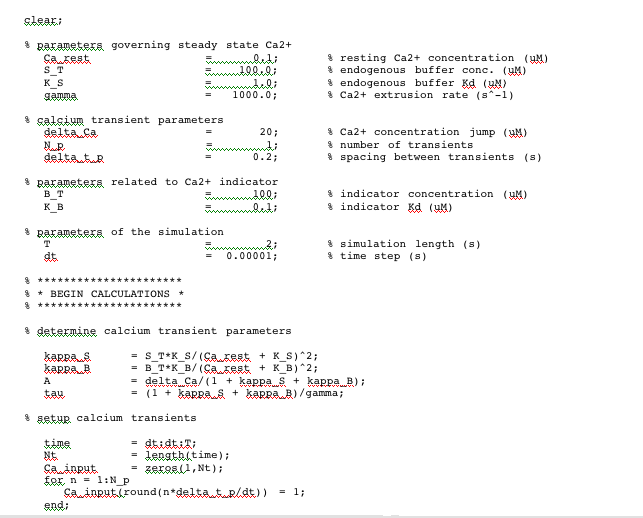
With this MATLAB excercise you will make calcium measurements in a model cell. Begin by downloading this document which includes all the directions and the MatLab program that follows.
Introduction
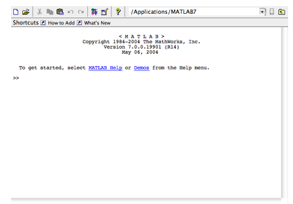
In this exercise, you will study concentration and binding dynamics of calcium in a sim-plified model of a cell. The exercise will be performed in Matlab, using a macro (“m-file” in Matlab terminology) called Ca_kinetics.m. To run the model, you will start Matlab on your computer. When the program opens, you will see a window titled “MATLAB” that looks like this:
The “>>” symbol is the command line prompt. Type “edit Ca_kinetics” at this prompt to open the modeling m-file in the default text editor. You should be able to scroll through the m-file to examine it. Do not edit it in any way yet. At the top of the editor window is a symbol:
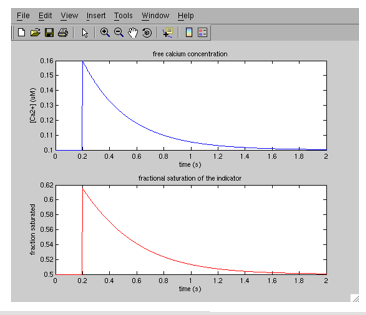
Clicking this symbol saves and runs the m-file; click it now. You now should see a new window titled “Figure 1,” that looks like this:
You can use the magnifying glass tools on the toolbar at the top to zoom in and out on either of the two plots. Double clicking with either one resets the plot. You can also type “grid on” at the command line to display grid lines on either subplot; select the subplot you want to do this in using the arrow tool in the figure toolbar.
Description of the model
The m-file we are using implements a so-called “single compartment” model of a cell undergoing calcium fluctuations; in other words, the cell is assumed to be a single, ho-mogenous container of reagents with no spatial variation of calcium or calcium-binding molecules. Calcium enters the cell in pulses called “transients,” each of which corresponds to injection of a fixed concentration of calcium (delta[Ca2+]T) at an instant in time. When calcium enters the cell, some is bound by endogenous proteins (approximated as a single species, S, with total concentration [S]T and dissociation constant KS); some is bound by exogenous fluorescent indicator (B, with total concentration [B]T dissociation constant KB); and some remains free ([Ca2+]free). Calcium is distributed to each of these three pools such that:
kS and kB are referred to as the “calcium binding ratios” for S and B, respectively. In reality, both kS and kB are calcium-dependent variables, but for purposes of our simplified model, we will approximate them as constants equal to their values at the cell’s resting calcium level, [Ca2+]rest. The dynamics of the system are then governed by the following equation:
This equation simply states that the change in calcium at any time (left side) is equal to the pulsed increase in calcium at times tp (right side, first term) minus the extrusion of calcium with rate constant g (right side, second term), where delta[Ca2+]free = [Ca2+]free – [Ca2+]rest. By solving this equation, we can determine the amplitude (A) and decay time (t) of the spikes in free and bound calcium caused by each injection. These are given by:
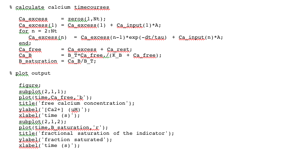
The model calculates these quantities and computes dynamics for a user-defined sequence of Np calcium input pulses with interpulse interval delta tp, beginning at t = delta tp. The full text of the m-file is given at the end of this handout. Two additional model parameters are T, the total length of the simulation, and dt, the “time step” used in calculating dynamics. The time step is necessary because the model really calculates a discrete approximation to continuous dynamics. A smaller dt will lead to a finer approximation.
The next section poses some questions you will answer as part of the exercise. Most of the questions will require you to run the m-file after resetting some of the parameters in lines 4-20 of the m-file. Each time you run the m-file, you will generate a new figure showing the trajectory of free calcium concentration (blue, top plot), and the fractional saturation of the calcium indicator (red, bottom plot). If you were doing actual fluorescence experiments, the signal changes you would be recording would be proportional to the fractional saturation of the indicator. In addition to learning about the calcium dynamics by reading the plots, you can learn the calculated values of each model parameter by typing the corresponding variable name at the Matlab command line:
Questions
1. Summation of calcium transients. Modify the default m-file to simulate the effect of 100 pulses, rather than just a single pulse. Also change the simulation length (T) to 10 seconds. Based on the Matlab-generated plot, what is the mean plateau calcium concen-tration (call it [Ca2+]plateau) observed after the cell reaches stead-state dynamics? With the default setting of Dtp = 0.2 s, the model simulates calcium pulses at a frequency (f) of 5 Hz. Plot [Ca2+]plateau vs. pulse frequency for Dtp = 0.1, 0.2, 0.3, and 0.4 s to show that [Ca2+]plateau = Atf + [Ca2+]rest. Why don’t A and t depend on f?
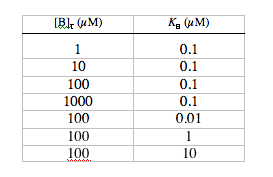
2. Dependence of dynamics on [B]T and KB. Return the m-file to the default settings. Without changing any of the other parameters, run the simulation with the following combinations of [B]T and KB:
Make a table showing values of A, t, kB, the maximum change in calcium indicator satu-ration (Dsmax), and the resting saturation level (srest), for each combination of [B]T and KB. Which of these conditions results in the greatest relative fluorescence change (µDsmax/srest)? Which results in the largest absolute fluorescence change? Consider t as a function of KB for all the conditions where [B]T = 100 µM; note that Dsmax is greatest when KB = [Ca2+]rest, and explain why indicators with significantly higher or lower values of KB would experience smaller changes in saturation. For “fast” detection of calcium transients (i.e., with minimum t), why is it better to use a low affinity dye than a high affinity dye? Add a column to your table, showing A times t for each condition. What do the values for At tell you about the dependence of [Ca2+]plateau on [B]T and KB?
3. Graphical determination of kS and g. Beginning from equation [5] above, derive an expression for t in terms of kB. With reference to this expression, use the data points you calculated in question 2 to demonstrate how values for kS and g can be determined from a plot of t vs. kB.
4. Limits of discrete simulation. The simulations you have been running have all used a discrete time step (dt) of one millisecond to approximate the dynamics of a continuously varying system. Starting from the default parameters, set the number of calcium pulses Np to 100 and the simulation length to 10 s. Run the simulation with time steps of 3 ms, 10 ms, 30 ms, 100 ms, and 300 ms, and make a table showing [Ca2+]plateau, as well as the maximum value of [Ca2+]free, for each dt. Note that at high values of dt, the calculated [Ca2+]plateau differs from the predicted values you determined in question 1. Now change [B]T to 10 µM and repeat the process, adding the new values of [Ca2+]plateau to your table. Considering the values of t and tp relevant to each of the simulations your performed, suggest and justify general criteria for choosing dt relative to t and tp, such that the dynamics of the system will be well modeled by the simulation.
5. Validity of model assumptions. A key assumption of the model we are implementing is that values of kS and kB are determined by [Ca2+]rest, but do not otherwise depend on calcium concentration. According to this assumption, the change in [BCa] due to a single calcium transient should be approximately kBD[Ca2+]free. An exact equation relating [BCa] to [Ca2+]free may also be derived using [B]T and KB:
In fact, it is this relationship that is used to compute the instantaneous values of fractional saturation ([BCa]/[B]T) reported by the simulation we are running. By comparing the changes in [BCa] predicted by the assumption of fixed binding fraction with values of [BCa] calculated using [B]T and KB, we can test the validity of the assumption. Return the simulation parameters to their defaults and run the simulation with delta[Ca2+]T set to 1 µM, 10 µM and 100 µM. Use the simulation output to determine the change in [BCa] predicted using binding fractions and using KB. Explain why the binding fraction estimate is worse for higher values of delta[Ca2+]T. What does this say about the model’s estimates of [Ca2+]free (also calculated using binding fractions)? What condition on [Ca2+] must be satisfied in order for the model to be effective at making predictions using binding fractions?
Part 2: Oral presentation instruction
DONE!
For next time
- Please download the midsemester evaluation form File:Macintosh HD-Users-nkuldell-Desktop-MidsemesterEval 20.109.doc. Complete the questionnaire and then print it out without including your name to turn in next time. If there is something you'd like to see done differently for the rest of the course, this is your chance to lobby for that change. Similarly, if there is something you think the class has to keep doing, let us know that too.
- Prepare a ten-minute oral presentation of a primary research paper related in topic to the experiments performed in this experimental. These presentations will be done individually. Some articles that are suitable for presentation are listed under the link for the next lab. These can be reserved on a first come/first served basis so email your choice as soon as you’ve decided, and then add your initials/lab section/team color next to the article so everyone will know it's been "taken." You can also search PubMed and identify a different article that you might prefer to present. In this case, please email the idea to Natalie for approval. Either way, email your finished presentation to Natalie, as the presentation order will be determined by the order they are received.

