User:Yeem/20.309/Mod 1 lab report
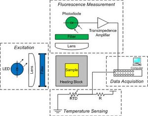
During the DNA melting curve module our goal was to construct a device to determine the effects of various parameters on the melting temperature of DNA. Samples were mixed with dye in cuvettes and heated in a water bath, then subjected to excitation by a filtered light source. The resulting fluorescence intensity was measured by a photodiode, whose signal was fed into a transimpedence amplifier. Voltage from the photodiode as well as from a resistance temperature detector were recorded by a PC data acquisition program and were analyzed by Matlab.
DNA melting curve apparatus
The circuit we devised was given to noisy interference and plagued by inconsistencies. Despite our best efforts, the system failed so often that we were at times highly suspicious of its output, even when it appeared to be operating correctly. Nonetheless we were able to gather useful data, with the help of multiple filters and smoothing.
Optical system
Our light source was an LED with a peak wavelength of 475nm. We used SYBR Green dye in our DNA samples, which is excited by blue light with a wavelength of 498nm. To narrow the spectrum of our LED, we used a Chroma Technology D470 filter; to narrow the cone of divergence, we used a lens with a focal length of 50mm.
SYBR Green dye emits light with a wavelength of 522nm. We attempted to minimize the effects of other light sources by using another filter and lens combination in front of our photodiode, and additionally mounting the fluorescence recovery tube at a ninety degree angle to the source of excitation.
Electrical system
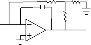
The aforementioned LED was driven with a constant current source provided by an LM317T variable voltage regulator. Current from the photodiode served as the input of an LF411 transimpedence amplifier with a gain of approximately 1e8 V/A. In addition, we connected a capacitor across the input and output leads, sacrificing time reponse for noise reduction. We used a potentiometer to remove the offset voltage by "zeroing" the pot for a dark input.
Measurements of temperature were done indirectly via an RTD mounted on the heating block cointaining our DNA sample. The RTD was connected to a voltage divider with 15[math]\displaystyle{ k\Omega }[/math] and 100[math]\displaystyle{ k\Omega }[/math] resistors. The voltage across the RTD was recorded in LabView.
Procedure
Our samples were prepared by pipetting 500uL DNA mixed with SYBR green dye into a cuvette and covering the surface with mineral oil to prevent evaporation. The cuvette was inserted into a heating block, then heated in a double boiler until it had reached a temperature around 90 degrees Celsius, as measured by the resistance of the RTD using a digital volt meter. At this point, we removed the heating block from the boiler and mounted it on our apparatus using the "quickconnect". The optical portion of the device was covered with a cardboard box and dark blanket to block out ambient light. The fluorescence intensity and RTD voltage were measured in LabView.
Methods
- Our Matlab m-files are available here.
Voltages from the transimpedence amplifier and the RTD circuit were sampled in real time with LabView. We took this tab-delimited raw data and attempted to filter out high-frequency noise by convoluting the voltage vectors of each sample with a low-pass filter kernel. Our kernel, [math]\displaystyle{ H }[/math], was specified in lowpass.m by
- [math]\displaystyle{ H = \{x | \forall n \in W (x = \frac{1}{\Sigma x} e^{\frac{-n}{k}})\} }[/math]
where [math]\displaystyle{ W }[/math] is the set of a sequence from 1 to the length of the kernel window and [math]\displaystyle{ k }[/math] is the exponential decay constant. For our filter, we used
- [math]\displaystyle{ W = \{1,2,...,16\} }[/math]
[math]\displaystyle{ k = 8 }[/math]
to define [math]\displaystyle{ H }[/math]. Our filtered output was characterized by [math]\displaystyle{ f * g }[/math]. To account for edge effects, we padded our raw data by appending [math]\displaystyle{ |W| }[/math] data points at the beginning matching our first experimental value and another set of data points at the end equal to our last data point.
At this point our sample data was stored in an [math]\displaystyle{ nx2 }[/math] matrix where [math]\displaystyle{ n }[/math] is the number of distinct time points. Next, we assumed that each experiment began with the sample completely dehybridized at 90 degrees Celsius and ended completely hybridized at 40 degrees C, and normalized our data accordingly. Theoretically we would have calculated our temperature directly via
- [math]\displaystyle{ R_L = V_m(\frac{V_i-V_m}{R_1} - \frac{V_m}{R_2})^{-1} }[/math]
- [math]\displaystyle{ R_L = R_0 + \alpha T }[/math]
- [math]\displaystyle{ T = \frac{1}{\alpha}[V_m(\frac{V_i-V_m}{R_1} - \frac{V_m}{R_2})^{-1} - R_0] }[/math]
in terms of
- [math]\displaystyle{ R_1, R_2 }[/math], the resistors in the voltage divider,
- [math]\displaystyle{ R_L }[/math], the temperature-dependent RTD resistance,
- [math]\displaystyle{ R_0 }[/math], the base RTD resistance,
- [math]\displaystyle{ \alpha }[/math], in units of [math]\displaystyle{ \frac{\Omega}{^{o}C} }[/math],
- [math]\displaystyle{ V_i }[/math], the input voltage,
- [math]\displaystyle{ V_m }[/math], the measured voltage drop across the RTD,
but our RTD voltage readings were inconsistent, as we had incorrectly constructed the voltage divider for some measurements. Therefore we assumed that we began with a fully heated sample at 90 degrees C and stopped with a fully hybridized sample at 40 degrees C. The script in relativetemp.m generates a set of values such that each temperature has been normalized on a scale of 40 to 90. relativefluro.m does the same for relative fluorescence.
The correctly scaled [math]\displaystyle{ nx2 }[/math] matrix is then fed into singlevalue.m which generates a bijection between each temperature value and the average of each fluorescence value at that point. We used a novel method to generate this relation, which was the source of great frustration.
Other assumptions we made included the linear correlation of DNA hybridization with relative fluoresence, as well as linear cooling of the RTD over time. Plots of fractional hybridization versus temperature were eyeballed and resampled with the Matlab function desample to further remove noise if necessary.
Finally, the discrete derivative of the relative fluorscence with respect to temperature (time) was taken and graphed on a separate chart. deriv.m performs a derivative by
- [math]\displaystyle{ \frac{df}{dT} = \frac{diff(f)}{diff(T)} }[/math]
where [math]\displaystyle{ f }[/math] is relative fluorescence, [math]\displaystyle{ T }[/math] is temperature, and [math]\displaystyle{ diff }[/math] is a function that returns the difference between sequential values in a vector.
tmelt.m is a script that generates a text label on each melting curve showing the coordinates of [math]\displaystyle{ T_m }[/math]; it was not used in these graphs as it tended to clutter the charts.
Results
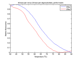
The plot of perfectly matched strands of DNA in figure 4a shows the reuslts we were expecting. In this graph, the response of relative fluorescence to temperature was vaguely switchlike and generally smooth. Changes in melting temperature were expected to cause simple translocations along the temperature axis, preserving the overall shape of our function. Figure 4a is void of obvious high frequency noise, drift, or other distortion.
Effect of ion concentration
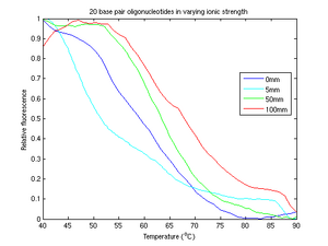
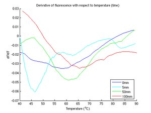
In figure 3, we recorded four runs of DNA samples with KCl concentrations of 0mm, 5mm, 50mm, and 100mm. The general trend appears to be increasing melting temperature with increasing ion concentrations. It seems that the 5mm curve is an abberation; its fluorescence curve is inconsistent with the general trend and its peak derivative is out of order. The data from the 5mm run was noisy; we were forced to resample. Unfortunately, even after resampling we were left with a significant drift, the cause of which we discuss later.
Effect of length
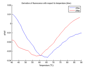
Of all of our experimental runs, the perfect match samples produced perhaps the best data. From figure 4b, two distinct peak derivatives are visible, resulting in a curve (figure 4a) shifted to a slightly higher melting temperature. From this we conclude that longer molecules of DNA have a higher melting temperature than shorter molecules.
Unknown oligonucleotides
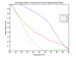
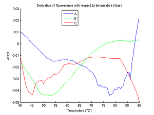
From figure 5, of the unknown samples, it is clear that B is the complete mismatch. The melting temperature of sample B is around twenty degrees lower than that of sample A. This suggests that one of samples A and C must be the perfect match and one must be the single mismatch. Unfortunately, the identities of A and C is difficult to resolve conclusively, due to fluctuations in sample C. Even after multiple experimental runs and much filtering and resampling, sample C continues to hinder us in our task of determining which sample is which.
Additionally, we cannot explain the fact that sample A has a concave shape (i.e., [math]\displaystyle{ \frac{d^2f}{dT^2} }[/math] is negative).
Theoretical model
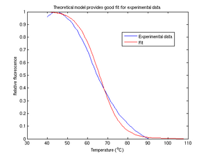
The theoretical model is calculated via
- [math]\displaystyle{ T(f) = \frac{\Delta H^{\circ}}{\Delta S^{\circ}-R \ln(2f/C_T(1-f)^2)} }[/math]
where [math]\displaystyle{ C_T }[/math] is the total concentration of single-strand oligonucleotides and [math]\displaystyle{ f }[/math] is the fractional hybridization calculated by normalizing photodiode voltage. In figure 6, we attempt to fit our data using coefficients for [math]\displaystyle{ H }[/math] and [math]\displaystyle{ S }[/math] solved by the Matlab function lsqcurvefit. The theoretical model appears to be a fairly reasonable fit for our experimental data.
Discussion
Our device was lacking in robustness. The data we gathered was at times noisy, inconsistent, or simply wrong. We experienced numerous setbacks, involving faulty circuit components, miscues in PC data acquisition, or human error.
Noise
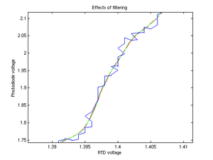
We employed numerous noise reduction mechanisms. At the most rudimentary level, during measurements we placed a cardboard box and dark blanket over our apparatus, in order to reduce the influence of ambient light on our measurements. Very high frequency noise was removed from the output of the transimpedence amplifier by connecting the input and output with a capacitor. However, in doing so we created another problem, in that the output was characterized by a significant time delay as the capacitor accumulated charge.
Whenever possible, we attempted to minimize the distance that wires had to run, and avoided crossing wires. Leads of circuit components were trimmed and kept short. We were sure to cover the BNC connection barrels with electrical tape. Power supply bypass capacitors bridged the all voltages and ground, and we connected our ground to the bench table. BNC cables were used for their shielding properties.
On the data analysis side, we noticed that portions of our curves had unexpected changes in derivative near the beginning and end of sample runs. These effects were attributed to the increased time delay of our RC circuit and eventual photobleaching of our samples. High frequency noise was removed by convoluting our signal with a low-pass filter kernel and resampling where necessary.
In spite of all this, many of our experiments were extremely noisy. When other groups in the lab had runs underway, we often noticed considerable drift in our measurements. On several occasions, a person merely walking by our device was enough to cause a jump in our measurement. Simple oversights such as failing to notice that a corner of the blanket covering our optical equipment had lifted up also caused us to repeat several samples.
Other problems
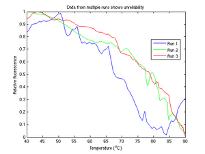
Despite our best efforts, our chief failure was the omission of sufficient testing prior to sample collection. Had we taken the time to double-check our circuit components, we might have been able to spot possible problems before they occurred. Our circuit's flaws were readily apparent when we performed pre-sample checkups on later runs.
For example, in attempting to ascertain the saturation voltage of the transimpedence amplifier, we aimed the desk lamp on our bench directly at our photodiode. Upon turning on the lamp, the output voltage began to behave erratically. We expected the voltage to saturate at a certain value and were surprised to find a wildly oscillating signal that had no apparent source. The phenomenon was reproducible to the extent that every time we switched the lamp on, our output lost all coherence. At a loss, we asked Rumi and Steve for help; eventually they were able to determine that our operational amplifier was unstable, and that the electromagnetic spike from turning on the desk lamp's circuit was causing our output to behave erratically.
The problem stemmed from our choice of resistors for the Sallen key feedback system in our transimpedence amplifier. Since we had inadvertantly chosen two resistors that had similar voltages, our circuit was highly unstable; this single error probably accounted for much of the headache that we experienced over the course of the module. The instability was such that regardless of what noise reduction methods we employed we were powerless to stop interference from something as innocuous a nearby desk lamp.
The op-amp instability was not our lone problem related to circuit construction. Our circuit behaved erratically at times when we placed our LED directly across our voltage source, drawing too much current. Once in a while our ground connection would become faulty, so we were sure to tape the underside of our breadboard and check the ground connection whenever began a day's work. The voltage divider connected to our RTD was mistakenly set up as several resistors in series, overloading the RTD with an influx of current. Other times, we were not to blame for circuit element failure; for example, an op-amp gave out even after we had fixed its stability issues.
We were often wary of the "differential" and "single-ended" settings on the LabView GUI and breakout box. Whenever we got an unexpected result, our first instinct was to check the channels to make sure all were switched to the same setting. Several runs were spoiled when a single switch was set to single-ended when the rest were differetial; we recommend that manufacturers replace individual switches with a single all-or-none switch.
Conclusion
The crucial role of circuit debugging prior to data collection has been drilled into us; we are now cognizant of its importance. In future experiments we will be sure to double- and triple-check our equipment to avoid gathering noisy, drifiting data. We would like to thank Rumi and Steve for all of their assistance, from demystifying voltage dividers to solving our opamp's stability issues. □