User:VisvaM/Notebook/Applications of Cell-Free Protein Synthesis and Biosensors to Metabolic Engineering

	<sitesearch>title="Search this Project"</sitesearch>
Customize your entry pages
Project Description Applications of Cell-Free Protein Synthesis to Metabolic Engineering The aim of this project is to explore how cell-free protein synthesis (CFPS) and cell free metabolic engineering (CFME) can be used to identify the concentrations of enzyme encoding DNA that lead to the maximum titre of a desired metabolite. Due to the COVID19 pandemic, this will be achieved by means of constructing computational models. Regarding the structure of the project work, the project will be split into two phases. Phase 1 In phase 1, the team will carry out a library-based investigation into the different metabolic engineering approaches that have been developed and explore the advantages and limitations of each. Additionally, the team will explore the difference between CFPS and CFME and the different modelling approaches that are used to model cell-free systems. The group will also identify a biosynthetic pathway that involves three to five enzymes and yields a metabolite which has significant potential to contribute towards the bioeconomy. The decision was made amongst the group to investigate a metabolite that not only has potential to contribute to the Bioeconomy, but specifically towards the aim of ‘manufacturing medicines of the future and making existing ones more efficiently’ outlined in the national bioeconomy strategy to 2030. Phase 2 In phase 2, the group will carry out modelling to assess how variations in the concentrations of the enzyme encoding DNA will impact the yield of the desired metabolite in a cell-free system. The other objective of this phase will be to explore how the modelling of CFME can be used to inform the design of in vivo metabolic engineering projects. References Introduction to the Team Our team is composed of 6 members, five 3rd year molecular bioengineers and one intercalating medical student. Molecular Bioengineers Olivia Hasson Aparna Loecher Visva Moorthy Edwina Rossi Stephanie Sze Intercalating Medical Students Celine Mark Positions of Responsibility Team Member Responsibility Olivia Hasson Project leader and supervisor coordinator Aparna Loecher Recording meeting minutes Visva Moorthy Wiki development Synthetic biology What is synthetic biology? A report published by the Royal Academy of Engineering proposed the definition that ‘synthetic biology aims to design and engineer biologically based parts, novel devices and systems – as well as redesigning existing, natural biological systems’ . Synthetic biology is an interdisciplinary field, encompassing engineering, biological sciences and modelling (Polizzi, 2013), and it is estimated that by 2025 the global market size for synthetic biology will be around $19.8 billion. One of the main aims of synthetic biology is to make the engineering of biological systems easier . Modularity is an example of one engineering principle which synthetic biology heavily relies on and this principle is outlined in the abstraction hierarchy of synthetic biology: biological parts (bioparts) are assembled to make up devices, which come together to form systems . Basic bioparts, which are the building blocks of synthetic biology, are defined as a functional unit of DNA that cannot be broken down into smaller parts . An article in Nature titled the ‘Five hard truths for synthetic biology’ highlighted that many of these bioparts haven’t been characterised well and even if they have the synergistic behaviour of these parts may diverge from what is expected . Thus, there is a big push to collect characterisation data for bioparts so that these parts are ‘fully characterised in the context of the hosts’ in which the experiments were carried out. International Genetically Engineered Machine (iGEM) and the Registry of Standard Biological Parts iGEM is a non-profit organisation whose main aims are to further the advancement of synthetic biology, education and competition and develop a collaborative and open community . iGEM hold a competition known as the iGEM competition which is aimed at students (teams are predominantly made up of university students). The Registry of Standard Biological Parts, run by iGEM, is a growing collection of more than 20,000 standard biological parts, which are referred to as BioBricks . A BioBrick is a DNA sequence that is flanked on either side by standardised sequences which encode restriction enzyme sites. References Introduction to Metabolic Engineering (ME) What is Metabolic Engineering? Metabolic engineering (ME) is defined as the ‘directed improvement of product formation or cellular properties through the modification of specific biochemical reactions or the introduction of new genes with the use of recombinant DNA technology’ . The applications of ME include the increased production of metabolites that are native to the host organism, the production of metabolites that are new to the host organism and the addition of pathways into the host organism that are able to degrade toxic chemicals . One of the main applications for which metabolic engineering is used, is to increase the production of a target metabolite . Prior to metabolic engineering, classical strain improvement was the method used to overexpress a desired metabolite; this involved mutagenesis carried out by a selection pressure such as UV light followed by screening of the resulting mutant strains. However, developments in recombinant DNA technologies led to a more rational approach to strain improvement known as metabolic engineering, which allows the ‘introduction of targeted genetic changes’ . In recent years, there has been a lot of attention towards the bio-based economy: a sustainable development concept that is concerned with using ‘renewable biological resources to replace fossil fuels in innovative products, processes and services’ . Metabolic engineering is concerned with the optimisation of titer, productivity and rate of metabolic pathways to create cost effective means for the production of fuels, chemicals and pharmaceuticals , which will ultimately accelerate the transition to a bio-based economy. One example that highlights the role of metabolic engineering in developing the bioeconomy is the successful production of a precursor of the anti-malarial drug, Artemisinin, using Saccharomyces cerevisiae . Artemisinin is derived from the leaves of the wormwood plant species Artemisia annua and is extremely effective in the treatment of drug-resistant Malaria . However, the Artemis annua plant only contains small quantities of Artemisinin and its chemical synthesis is not economically viable . Paddon et al were able to demonstrate high yields of 25g/l of the precursor, artemisinic acid, as well as develop a means of the conversion of artemisinic acid to Artemisinin. With support from the Bill and Melinda Gates foundation, this innovative application of metabolic engineering led to the delivery of 120 million treatments of Artemisinin-based combination therapies (ACTs) . Traditional metabolic engineering involves the use of microbial cells as cellular factories . The use of microbial cells in this way presents many challenges which include slow design-build-test cycles due to the constraints of cellular growth, toxicity of metabolites to the host organism and an inability to steer resources towards the synthesis of the target metabolite . One of the main disadvantages of in vivo metabolic engineering is the balance that exists between the engineer’s objectives (often the overexpression of a target metabolite) and the cellular growth objectives . A nature communications article by Tsutomo et al, recently reported the development of a new metabolic engineering strategy called Parallel Metabolic Pathway Engineering (PMPE) . PMPE was able to use the two different sugars found in Lignocellulosic biomass, xylose and glucose, for two different objectives: glucose was used for the production of the target metabolite, muconic acid, and xylose was used to propagation of the E. coli bacteria . In this way, PMPE was able to independently control bacterial propagation and target metabolite production. Another metabolic engineering strategy that overcomes many of the aforementioned limitations of traditional in vivo metabolic engineering is Cell-Free Metabolic Engineering (CFME), which unlike PMPE, completely eliminates the concern regarding cellular growth. References What is Cell Free Metabolic Engineering (CFME)? Cell-free metabolic engineering (CFME) enables the synthesis of metabolites outside the confines of the cell, by exploiting cellular machinery. This approach decouples cellular growth objectives from the engineer’s objective to optimise the production of a particular metabolite . CFME offers many advantages over traditional in vivo metabolic engineering. These include enabling the synthesis of metabolites that are toxic to living cells, facilitating the real-time monitoring of intermediates and a greater ability to manipulate reaction conditions. Additionally, cell-free systems offer the potential to direct resources towards a desired metabolite .Within CFME, there exist two different synthesis systems: Crude Cell Lysate Systems and Purified Enzyme systems. Limitations of Cell Free systems One of the aims of the project is to explore how the modelling of cell-free metabolic engineering can be used to inform the design of in vivo metabolic engineering projects. However, cell free systems have many characteristics that make them inherently different from their in vivo counterparts. A perspective by Laohakunakorn highlights some of these characteristics, which include a lack of compartmentalisation, (due to the absence of cellular membranes in cell-free systems) the tendency of cell-free systems to approach equilibrium and the issue of resource depletion . The absence of compartmentalisation results in a reduction of molecular crowding . Molecular crowding limits diffusion of macromolecules , which suggests that the kinetics of a cell-free system and in vivo system will be different. This raises the question of to what extent can insight obtained from cell-free systems be meaningfully applied to in vivo systems? Crude Cell Lysate Systems Crude Cell Lysate systems are prepared by cell lysis followed by the removal of cellular debris . Cell lysates present some advantages over purified enzyme systems including the ability to recycle energy and the preservation of native metabolic pathways from the host cell which can support cofactor regeneration . Additionally, cell lysates are very cheap to obtain whereas the purification of enzymes required for purified enzyme systems are associated with high costs. Extensive research has been directed towards the optimisation of crude cell extracts. In particular, Jewett et Al have shown that more efficient protein synthesis can be achieved by removing unnatural components (e.g. pH buffers) from the cell lysate and more closely mimicking the cytoplasmic composition of the host cell . Purified Enzyme Systems Purified enzyme systems are obtained by an overexpression of enzymes in distinct cells, followed by the subsequent purification of these enzymes . One advantage of purified enzyme systems is that they are not subject to the undesired ‘background metabolism’ that is present in crude extract systems and which can make the system difficult to model. Purified enzyme systems offer a much greater degree of control over pathway fluxes due to the fact that the concentration of every component is known (. However, the limitations of purified enzyme systems include the high cost of cofactors, which are required for enzyme activity, and the issues associated with cofactor regeneration. References Difference between Cell Free Protein Synthesis (CFPS) and CFME The distinction between CFPS and CFME is that the objective of CFPS is the engineered production of a protein. On the other hand, CFME is concerned with the production of target metabolites using in vitro combinations of enzymes, which have been obtained either from crude cell lysates or enzyme purification processes. The aim of our project is to select a metabolic pathway that produces a metabolite that has the potential to contribute towards the field of healthcare within the context of the bioeconomy. Ideally, we are aiming to model CFPS that will produce the constituent enzymes that are involved in the metabolic pathway and then proceed to model the resulting metabolic network using CFME. This metabolic engineering approach is referred to in the literature as cell-free protein synthesis driven metabolic engineering (CFPS-ME) . CFPS-ME further increases the DBT cycles by synthesising the enzymes involved in the metabolic pathway in vitro using CFPS which eliminates the need to culture cells to individually overexpress each enzyme. Additionally, it eliminates the requirement of enzyme purification that is present in the construction of purified enzyme systems. The ability to use CFPS-ME for rapid prototyping was highlighted in a study conducted by Jewett et al, who, in the space of a single day, were able to test several different enzyme homologs to try and optimise n-butanol production. However, attempting to reconstruct the entire n-butanol synthesis pathway using CFPS-ME, they found that as they increased the number of enzymes produced by CFPS the amount of n-butanol produced decreased. References Metabolic Bottlenecks Metabolic bottlenecks in metabolic engineering refers to the capacity of the system being limited by a single component ie. metabolite of the pathway. This term, when applied to metabolic engineering, suggests that a single synthetic pathway puts a constraint on the production of the end-product metabolite. In a given metabolic reaction network, there will exist bottlenecks which can massively decrease the yield of the final desired metabolite; Additionally, the presence of bottlenecks in the metabolic pathway can result in an overproduction of the intermediate metabolites, which could elicit a stress response in the cell. This forms the basis of a major disadvantage of in vivo metabolic engineering. Common metabolic bottlenecks include the local accumulation of toxic intermediates or byproducts, cofactor imbalance and inefficient enzymatic activities. By identifying these metabolic bottlenecks, one can attempt to design a metabolism pathway that overcomes these metabolic bottlenecks in order to increase the yield of the final desired metabolite. However, the complexities of these pathway designs remains a significant challenge for metabolic engineering. References Metabolites Antivirals Seasonal Influenza “Seasonal influenza can infect up to 20% of the population. Up to 650000 people die of respiratory diseases linked to seasonal influenza each year and up to 72000 of these deaths occur in the WHO European Region.” In the context of the bioeconomy, the burden of influenza is tremendous in the form of medical care, healthcare utilization and lost working hours. There are four types of influenza viruses with Influenza A and B viruses causing seasonal epidemics of disease. Structure of Influenza Virus and Viral life cycle Although the structure of the influenza virus can vary, there are two different glycoprotein spikes embedded on the viral envelope: hemagglutinin (HA) and neuraminidase (NA) proteins. Within the lipid envelope is the influenzas’ genome, organized into eight pieces of single stranded RNA. The viral life cycle can be segmented into the following stages: viral attachment to host cell, viral penetration into host cell, viral uncoating, viral genome replication and transcription, viral translation and assembly followed by viral progeny release. Influenza virus first recognize and bind onto the sialic acid sugars on the surface of the host cell through HA, which triggers a merging of the viral envelope with the host’s endosomal membrane, allowing the viral ribonucleoprotein (RNP) complex which consists of viral RNA segments coated with nucleoprotein and RNA polymerase to enter the host’s cytoplasm through endocytosis. RNPs then enter the host cell nucleus where mRNA of viral origin can be exported and translated. After budding of the influenza virus is complete where mature virions bind on the sialic acid as before through the HA, they detach from the cell surface due to the sialidase activity of the NA protein. The NA protein cleaves terminal sialic acid residues from the cell surface to release progeny virus from the surface of the host cell as well as removes sialic acid residues from the virus envelope itself to prevent viral particle aggregation, enhancing infectivity. Lastly, NA also plays a role in allowing virions to enter respiratory epithelial cells by breaking down mucins in respiratory tract secretions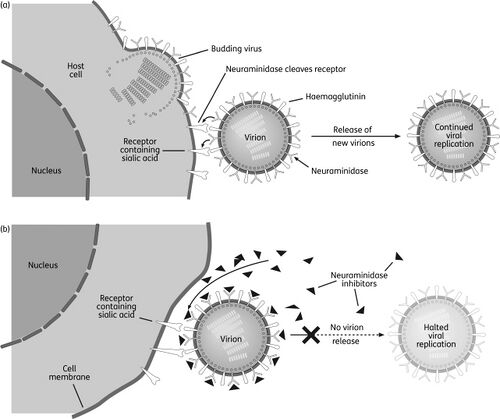. Shikimic acid and Tamiflu Oseltamivir (sold under Tamiflu) is in a class of medications called neuraminidase inhibitors and aids in preventing and treating influenza A and B. It is ingested in the form of an oral prodrug, oseltamivir phosphate, a compound that is metabolized in the body by hepatic esterase into its pharmacologically active form, oseltamivir carboxylate (OC). It binds to and inhibits the active site of the neuraminidase enzymes that plays a significant role in the release of progeny viruses and enhancement of infectivity, as mentioned above. OC effectively reduces viral replication, limits viral load, drastically reducing influenza symptoms and associated complication. Because of the highly conserved active site of the neuraminidase enzyme, it is effective against all neuraminidase subtypes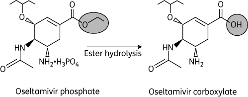. Shikimic acid is an important intermediate for the manufacturing of oseltamivir, along with other pharmaceutical compounds. These include Zeylenone and 3,4-Oxo-isopropylidene-SA that has antiviral, anticancer, antibiotic properties and antithrombotic and anti-inflammatory effects, respectively. Shikimate, the more commonly known anionic form of shikimic acid, is naturally extracted from the pods of Chinese star anise plants; however, inadequate raw feedstocks and the complex extraction that involves a 10-step process that takes approximately 6-8 months to complete have rendered it challenging to meet the worldwide demand for it. Chemical- based synthesis are also commercially unattractive because of environmental concerns.. Therefore, there is an ever -increasing demand for an alternative synthesis method for elevated shikimate production. The shikimate pathway is found in bacteria, fungi, plants and algae and is shown in the diagram below. It begins with the condensation of intermediates of the glycolytic pathway and the pentose phosphate (PP) pathway, phosphoenolpyruvate (PEP) and erythrose-4-phosphate (E4P), respectively. These two pathways are part of the central carbon metabolism (CCM), consisting of enzymatic reactions that convert carbon sources into biomass energy. These two compounds are initially combined to produce 3-deoxy-D-arabino-heptulosonate-7-phosophate (DAHP) by DAHP synthase. In E.coli, there are three DAHP synthase isozymes – aroF, aroG and aroH. Hence the resultant DAHP is converted to shikimate with reactions catalyzed by these enzymes. These three isozymes are feedback inhibited by one of the end products, namely aromatic amino acids- tyrosine, phenylamine and tryptophan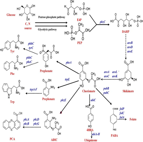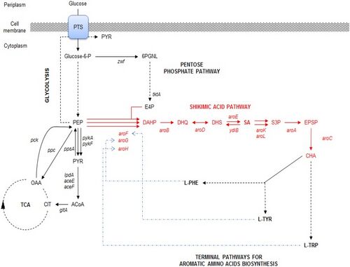. Antivirals - Figure 1. Shows the Interaction between CCM (PP, TCA, Glycolysis) and the shikimate pathway (upper) (lower) Metabolic Engineering Metabolic Engineering offers a solution to enhanced shikimate biosynthesis by blocking pathways that consume precursors of shikimate as well as overexpressing key genes of enzymes that play a role in its biosynthesis, increasing and directing flux towards the production of shikimate. The main metabolic engineering approaches have been based on genetic manipulations of the CCM and shikimate pathways. The fluxes of PEP and E4P can be increased through genetically engineering the glycolytic and PP pathways, respectively. Previous studies have shown the overexpression of transketolase (tktA) gene has contributed to an elevated concentration of E4P leading to a shikimate yield from 38 to 52 g/L. Other studies have shown that the overexpression of phosphoenolpyruvate synthase (ppsA) involved in gluconeogenesis have also increased shikimate level to 71 g/L. The flux of PEP directed towards the shikimate pathway is often constrained due to the phosphotransferase (PTS) system, the method used by bacteria for sugar uptake where the source of energy is PEP. Hence, genetically modifying the PTS system or utilizing a different glucose transport system or other sources of energy such as pyruvate or glycerol have also been used to increase the yield. Another method that has been used is modifying the feedback resistance enzymes of the DAHP synthase isoenzymes. By eliminating the pathway regulators, the aromatic amino acids or by engineering the enzymes to be feedback-resistant, the yield can also be drastically increased. Overexpression of these three rate-limiting enzymes can also lead to a high level of synthesis of shikimate. Potential of Cell-Free Metabolic Engineering Although there have been no published studies on conducting cell- free metabolic engineering to increase the yield of shikimic acid. There are many advantages and disadvantages to employing a cell-free approach, outlined below. Cell- free systems bypass cell growth, permitting more DBT cycles and avoids the conflict of resource allocation between cell growth and biosynthesis of target products. The open environment allows for direct modification of the components in the reaction. CFPS-based metabolic engineering where gene cloning, bacterial transformation, in-vivo protein expression, cell lysate preparation and protein purification are eliminated to further bypass cell growth, drastically shortening DBT cycles. L-DOPA Significance of L-DOPA in the Bioeconomy L-DOPA is commonly used as a Parkinson’s treatment. The production of L-DOPA has a substantial market size of 3.99 Billion USD as of 2016 . This value has an expected Compound Annual Growth Rate (CAGR) of 6.5% from 2017 to 2022 to ultimately achieve a larger market size of 5.69 Billion USD by 2022. Traditional Production of L-DOPA The conventional commercial production of L-DOPA is chemical synthesis with asymmetric/ enantioselective hydrogenation. L-DOPA - Figure 1. Enantioselective hydrogenation of C2-symmetric diphosphine with Rubidium catalyst to form L-DOPA The major limitations of this method is the poor conversion rate and low enantioselectivity. The poor conversion rate is attributed to the complicated reaction procedure that has to be conducted under very strict and harsh operational conditions, with low substrate specificity. Moreover, the reaction requires Rubidium as a metal catalyst, which is costly. Biotechnology Production of L-DOPA Biotechnological approaches have been explored as alternatives, with the goals of improving the reaction conversion rate and enantioselectivity, as well as economizing the production of L-DOPA. A method used is microbial fermentation. However, there are many limitations with these methods. The following are the microbial fermentation methods and their limitations: Tyrosinase in Asperigillus oryzae and/or Acremonium rutilum: Microorganism activity of tyrosinase is weak Target metabolites are rapidly decomposed Stoichiometric formation of L-DOPA is hard to achieve. Tyrosine phenol-lyase (TPL) in Erwina herbicola: Induction of TPL requires high levels of tyrosine, which is costly and also results in complex purification Tac promoter to induce high levels of TPL in absence of tyrosine High substrate concentration denatures the enzyme, thus requiring frequent additions of low concentration of substrates Complex purification p-hydroxyphenylacetate 3-hydroxylase (PHAH) in E. coli Need NADH as cofactor, which is costly The following are the overall limitations of biotechnological approaches: Time consuming: Compared to chemical synthesis microbial fermentation usually exhibits outstanding enantioselectivity, but it is a time-consuming process that takes over 10 days including the cell-culture period Complex purification: it is not easy to purify L-DOPA from culture media including analogous substrates such as L-tyrosine. Not necessarily cheaper than chemical synthesis: due to the high amounts of substrate and cofactor required, it is not necessarily cheaper than chemical synthesis Low yield: low productivity, low conversion rate, and denaturation of the biocatalyst Metabolic Engineering of L-DOPA The L-DOPA production depends on: availability of L-tyrosine & effective enzyme to catalyze the hydroxylation process. There has been an attempt of producing L-DOPA from L-tyrosine from glucose with glycerol using E. coli using metabolic engineering. In order to overcome the metabolic bottleneck, there was an introduction of feedback resistant enzymes, deletion of competing pathways, enhancement of catalytic activity of hpaB, and overexpression of critical pathway enzymes. To address the concerns about metabolic flux, carbon flux was channelled towards L-tyrosine production. This method of production allowed for a three times higher titre of L-DOPA from glucose with glycerol compared to previous works. However, the overexpression of relevant enzymes to increase the carbon flux in E.coli resulted in increased acetate production, which is toxic to the cellular health of E.coli. This limitation calls for the need for cell free metabolic engineering approaches to synthesised L-DOPa, which has yet to be explored. Carotenoids Introduction As outlined by the World Health Organization, “Vitamin A deficiency remains the single most important cause of childhood blindness in developing countries” – whilst also significantly contributing to morbidity and mortality rates infants of low-income countries . This health problem, which in fact is prevalent in more than half the countries of the world, is primarily caused by a lack of provitamin Vitamin A in the diet, and may be exacerbated by high rates of infection. Indeed, as humans cannot naturally synthesise Vitamin A themselves, it must be supplied through the diet by compounds known as carotenes, a subclass of carotenoids. Carotenoids, also known as terpenoids, are a group of naturally occurring compounds. Initially identified as colourants, these compounds collectively form the basis for a class of red, orange and yellow pigments widely found in nature . Though often considered to be plant pigments, they are also of crucial significance to numeral biological functions in the human body . Their physiological importance and their potential application for the prevention of conditions such as cancer, cardiovascular diseases, cataracts and other degenerative diseases have led to a growing demand for efficient and cost-effective production methods. In 2019, the global carotenoids market was valued at USD 1.5 billion and it is projected to grow to USD 2.0 billion by 2026. This significant market growth may be linked to the growing use of carotenoids in preventative healthcare, the increased use of carotenoids as food colourants and the emergence of new technologies for the extraction and synthesis of natural carotenoids . In the context of our project, the development of a model for cell-free synthesis of carotenoids could be of great potential value to the UK bioeconomy, given their vital significance in treating nutritional and age-related conditions. The Chemistry and Function of Carotenoids To date, over 1100 carotenoid compounds have been identified from various species of bacteria, eukaryotes and some archaea. Some commonly known carotenoids include lycopene, β-carotene, lutein, astaxanthin and canthaxanthin. As a subclass of isoprenoids, carotenoids are built from C5 isoprene units and rearranged to form long-chain C40 carotenes or xanthophylls – the two main groups of carotenoids. Carotenes are strictly hydrocarbons. Xanthophylls differ from carotenes in that they contain oxygen in addition to hydrogen and carbon, thus having functional groups such as alcohols or carbonyls. Carotenoids can also be grouped according to their structure. As outlined by Perera, C. O. et al, “carotenoids may be acyclic (e.g. lycopene) or contain a ring of six carbons at one or both ends of the molecule (e.g. β-carotene)”. It is indeed these different characteristic chemical structures that give rise to the physiological functions of carotenoids as antioxidants, provitamin A nutrients, and UV protection agents. Carotenoids - Figure 1 shows some major food sources of different carotenoids. 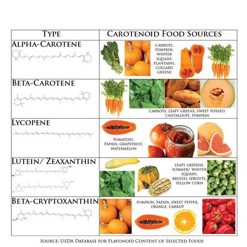Carotenoids - Figure 1. Carotenoid Food Sources Traditional synthesis of Carotenoids Plant Extraction Carotenoids were traditionally obtained through plant extraction methods based on physiochemical processes. Depending on the carotenoid of interest, different plants or vegetables may be used for extraction. As an example, the orange carrot is the most popular plant source for extraction of β-carotene, having up to 9.9932 mg beta-carotene per 100 g edible carrot. However, there are several disadvantages associated with the use of physiochemical extraction methods for carotenoids, including high costs, seasonal and geographical availability of the raw plant materials and the low yield of carotenoid per kg of plant material processed. Chemical synthesis Methods for chemical synthesis of carotenoids were developed in the 1905s and have since been used as an alternative to plant extraction. For chemical carotenoid synthesis, either Witting reactions or Grignard compounds are used. Witting reactions involve the production of aldehydes from aldehydes or ketones, whereas synthesis through Grignard compounds makes use of organometallic Grignard compounds. Though still widely used, some studies have shown that chemically produced carotenoids, such as synthetic beta-carotene, exhibit carcinogenic activity . Metabolic Engineering for Carotenoid Synthesis The limitations of natural extraction and chemical synthesis of carotenoids led to the application of metabolic engineering methods as an alternative production route to meet the growing demands from industry. As well as overcoming several of the challenges linked to natural extraction methods, the production of carotenoids through native microbial hosts also enables the use of low-cost substrates and the development of competitive bioprocesses. Many efforts have been made to genetically engineer microbial hosts such as E.coli and C. cerevisiae for the production of various carotenoids including lycopene and β-carotene. A review of the literature shows that many of these efforts involve optimising the biosynthetic pathway native to the host of choice. Others have successfully attempted to introduce the pathway into non-native hosts. To understand how metabolic engineering may be applied to carotenoid synthesis, a brief explanation of the carotenoid biosynthetic pathway is outlined below. Biosynthetic pathway of carotenoids As outlined by Wang. C et al., “the carotenoid biosynthetic pathway, native to several eukaryotes, bacteria and some archaea, can be divided into four steps: geranylgeranyl diphosphate (GGPP, C20) precursor supply, phytoene desaturation, lycopene cyclization, and carotene modifications”. A summary of these steps can be seen in Carotenoids - Figure 2. 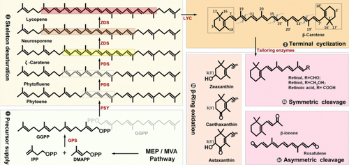Carotenoids - Figure 2. The Carotenoid Biosynthetic Pathway Supply of GGPP is achieved through two different isoprenoid pathways: the mevalonate (MVA) pathway native to eukaryotes and some bacteria and the non-mevalonate (MEP) pathway native to most bacteria and some plant plastids. Both of these pathways are involved in the synthesis of the two isoprenoid precursors DMAPP (dimethylallyl diphosphate) and IPP (isopentenyl diphosphate), of which one DMAPP and three IPPs are condensed to form one GGPP in a series of reactions. Several subsequent steps involving phytoene desaturation lead to the synthesis of the first carotene: lycopene. From here, different lycopene cyclases catalyse the introduction of a β- or ε-ring at the chain ends of lycopene to form α-, β-, γ- or δ-carotene, depending on the position of the ionone ring . Finally, these carotenes can be hydroxylated at the terminal ionone ring by hydroxylase and ketolases to form various xanthophylls such as zeaxanthin, canthaxanthin or astaxanthin. Metabolic Engineering of Carotenoids In efforts to produce carotenoids through in vivo metabolic engineering of microbial hosts, several methods have been tested and evaluated. As outlined in a review by Li, M. et al., efforts to produce lycopene through metabolic engineering of E. coli have involved a variety of optimisation strategies. These include but are not limited to: Overexpression of carotenogenic (crt) genes in non-carotenogenic organisms Adjusting the copy number of crt genes to direct more metabolic flux to the lycopene biosynthetic pathway Optimisation of the native metabolic flux of the MEP pathway Exogeneous expression of the MVA Pathway Sufficient support of precursor and cofactor Membrane engineering to improve permeability and storage capacity of membranes Overall, the ease of genetic manipulation, rapid growth and simple media requirements make microbial hosts such as E.coli good candidates for the in vivo production of lycopene, as well as other isoprenoids. However, the extraction of carotenoids produced in microorganisms remains a complicated and expensive process. Long-chain hydrophobic carotenes such as lycopene typically accumulate in membrane compartments , thus complicating the extraction process. Indeed, studies have shown that high lycopene contents lead to membrane stress as excess lycopene accumulates in the cell membrane. This challenge highlights the possible need for cell-free methods in the biosynthesis of natural carotenoids – where extraction processes are easier and the accumulation of lycopene in membranes would not occur. The Potential for Cell-Free Synthesis of Carotenoids Though recent literature is scarce of studies that have attempted cell-free synthesis to produce and increase the yield of carotenoids, there may be several advantages of producing carotenoids through such an approach. Besides the aforementioned ease of extraction and overcoming the issue of cell membrane stress, CFME also allows for reduction of DBT (Design-Build-Test) cycles, operational simplicity, high conversion yield and productivity, quantitative and precise assessment of performance and greater design flexibility . References Modelling Introduction The goal of metabolic engineering is to develop targeted methods to improve the metabolic capacities of industrially relevant microorganisms, and mathematical modelling is a very successful scientific tool that can be used to achieve this . A mathematical model is an ‘abstract representation of a target system’ and one of its purposes is to ‘simulate, predict and optimize procedures, experiments and therapies. These models are used to understand internal and external cell interactions and how they influence cell metabolism. Specifically, processes such as metabolite concentrations and reaction fluxes of metabolic pathways regulated by enzymes under varying internal and external conditions are examined and translated to numerical problems with formal representations. This resulting model should have a high level of accuracy and detail in order to represent the complexity of the behavior of a metabolic network. Developing a computational model that simulates a metabolic pathway after, for example, the knockout of a component is very useful, since this process is much more difficult, time-consuming, and costly to carry out experimentally. For cell free systems, we can use modelling to simulate the outcome of metabolic pathways in order to predict and optimize the yield of a desired metabolite. There are two approaches for mathematically representing biological networks: stationary modelling examines the system at an equilibrium point where metabolite concentrations are constant over time. Dynamic modelling takes into account the changes in metabolite concentrations over time. Overall, depending on the extent of a models’ abstraction, it has a particular granularity, which refers to the level of detail in the description of the system. The choice of its level has many tradeoffs and considerations including cost and time-benefits. The accuracy of a model is limited by its granularity, and as George Box said “Essentially, all models are wrong, but some are useful”. Overall Framework for metabolic engineering The overall modelling framework begins with reconstructing the model from its genome sequence, information from biological databases and also literature. The model created can include stoichiometric information only or it can be incorporated with kinetics. Then the model is simulated for prediction of the phenotype of the system. For kinetic methods, steady and transient state behaviors of metabolite concentrations and fluxes are computed, while for stoichiometric methods, a flux distribution imposed by constraints is calculated. Lastly, the phenotype is evaluated and optimized until it meets termination criteria. The optimization includes integrating solutions as perturbations to the model, by changing the kinetic parameters or constraints so that a new phenotype can be simulated. Constraint Based modelling (CBM) Constraint based modelling framework is an approach to predict metabolic phenotypes in the stationary case, and limits models to only encompass reaction stoichiometry and reversibility. Thus, it is established on the assumption of steady-state operation and cannot express transient behaviours.The module formulations employed in this approach are based on linear equation systems that are normally undetermined, resulting in infinite solutions. For this reason, restrictions or ‘constraints’ and assumptions or ‘objective functions’ are implemented to identify the ideal solution. These rely on physical and chemical restrictions including fluxes, mass balance and thermodynamics and produce solutions that are characterized by steady-state flux distributions within the space of feasible solutions known as the flux hyper cone. The CBM method does not require any mechanistic knowledge, only minimum and maximum flux bounds are needed since changing metabolite concentrations over time and transient behaviors are not taken into account. CBM thus circumvents difficulties associated with estimating kinetic rate equations and parameters but still produces results that are usually close to experimental observations. The most common approach in identifying the optimal value for the flux distribution is Flux Balance Analysis (FBA), which examines the internal metabolite concentrations in a quasi-steady state and imposes specific constraints. FBA defines a linear, biological objective function relevant to the problem and optimizes it through minimization or maximization to determine the optimal flux distribution. FBA calculates the flow of metabolites through a metabolic network; thus, it can predict the growth rate of an organism or the rate of production of an important metabolite. Specifically, the first step of FBA is to metabolically reconstruct the network that is made up of a list of stoichiometrically balanced biochemical equations. The reconstruction is then mathematically modelled, which is done by creating a stoichiometric matrix (S), representing the metabolic reactions, of size m*n, where every row m represents a metabolite or compound (the system has m compounds) and every column representing a reaction (the system has n reactions). The entries in each column are the stoichiometric coefficients of the metabolites engaging in each reaction that implement restrictions on the flow of metabolites through the network. A negative coefficient is used for each metabolite that is consumed, a positive coefficient represents a metabolite that is produced and a coefficient of zero is employed for metabolites that do not take part in a certain reaction. The flux through all the reactions in a network is captured by the vector v, with a length n and the concentrations of metabolites are represented by the vector x, with length m. Since the system assumes internal concentrations of metabolites do not change over time , the system of mass balance equations at the steady state with dx/dt = 0, is Sv = 0. These constraints result in a range of solutions, however since there are more reactions than metabolites in most realistic models, there is more than one unique solution to the equation. Thus, the next step is to identify an objective function Z = cTv, c being a vector of weights representing how much each reaction contributes to the objective function . The system is then optimized via linear programming and the output is a specific flux distribution v that maximizes the objective function. The COBRA Matlab Toolbox can be used to carry out necessary calculations. Dynamic Modelling Dynamic modeling describes cell metabolism using methods based on the kinetics of metabolic processes and produces detailed, unique solutions in time for both the transient and equilibrium states, starting from any initial metabolite concentration. It is based on knowledge of enzyme mechanisms and experimental data and can represent changes in metabolite concentrations over time through the use of ordinary differential equations (ODEs). The ODEs encompass initial metabolite concentration values, reaction rate equations and kinetic parameters. The solution spaces of dynamic approaches are a subset of constraint-based solutions, as they impose kinetic derived constraints on top of the same core constraints. In order to create a dynamic model, the first step involves establishing the interaction mechanism of the network and then secondly, the type of representation for the kinetic rate expressions needs to be decided [4]. After this, the model can be expressed by a set of ODEs that depict the time trajectories of the processes and output values that can be supplemented with experimental data. In order to build dynamic models, there are two approaches taken: bottom-up modeling integrates isolated pathway components obtained through mechanistic descriptions of behaviors to build the model and then uses experimental data to validate the model, involving many kinetic parameters [4]. On the other hand, building the model via a top-down approach employs experimental data to improve pre-existing models, allowing for the integration of unidentified mechanisms, interactions and properties into the model. Dynamic models can be subdivided into deterministic and non-deterministic models. There are two kinds of deterministic models, mechanistic and approximate kinetic models. Mechanistic models These models are based off mass action law, which explains that the reaction rate is proportional to the concentration of the reactants. Mechanistic expressions are employed for one-step reaction or their combination of their mass actions into multi-step reactions. Michaelis-Menten models are used to model enzymatic equations that do not have allosteric effects i.e. when a ligand binds to the enzyme which changes the properties of another site on the protein. Assumptions that are made for this model include Quasi steady state approximation that states that the concentration of the enzyme substrate (ES) complex is constant, meaning we assume that the enzyme concentration is much smaller than the initial substrate concentration leading to saturation of the enzyme. Conservation laws are also assumed, i.e. that no enzyme is consumed or produced. The following equation is used to express the rate of the enzymatic reaction: [math]\displaystyle{ v_0 = \frac{d[P]}{dt} = v_{max} \frac{[s]}{[s]+k_m} }[/math] where v is the reaction rate, [S] is the concentration of the substrate, [P] is the concentration of the product, Vmax is the maximum reaction rate reached by the system, and km is a constant that represents the substrate concentration where the reaction rate is half of its maximum rate. Hill rate laws are used when cooperative binding is involved in the reaction, i.e when an enzyme has many binding sites and after binding of a molecule, the affinity of the enzyme changes. The hill equation is the following: [math]\displaystyle{ v_0 = \frac{d[P]}{dt} = v_{max} \frac{[s]^n}{[s]^n+k_m} }[/math] Thus, when the order n=1, the hill equation is the same as the Michaelis-Menten equation. Approximate Kinetic Models These models aim to describe the behavior of biological systems using only a small number of defined parameters. This is useful since reliable rate equations required by mechanistic models are not always known for certain reactants and the rate expression can be challenging to quantify. These models are ‘approximate’ because they exhibit similar model behavior to mechanistic models with respect to transient and steady states but with fewer parameters. Linear-Logarithm (Lin-Log) Kinetics are used in gene regulatory systems where rates of enzyme reaction are proportional to enzyme concentration and can produce analytical solutions for the steady states. They work best modelling systems that undergo exponential growth and have been proved to model in-vivo systems accurately. The equation for this can be seen in Modelling - Table 1. Log-Linear (Log-Lin) Kinetics are used in metabolic where parameters are influenced by spatiotemporal variations. This approach is very similar to Lin-Log in that it results in analytic solutions by imposing linear and logarithmic expressions, however for Log-Lin the reaction rate is not proportional to the enzyme concentrations. Thus, it can be employed to represent dynamic systems with strong nonlinearities. However, this model uses quasi steady state approximation, which assumes that all state variables are constant meaning it is not suitable for transient systems. Power laws are used to simply model aggregation and consumption processes in enzyme catalyzed reactions and can calculate analytical solutions at the steady state. It has the equation seen in Modelling - Table 1. Convenience rate laws are used to thermodynamically, independently represent enzyme saturation and regulation through activators and inhibitors. It is a general form of Michaelis-Menten kinetic which incorporates stoichiometries and assumes a fast equilibrium between substrates, products and enzymes. It assumes an enzyme mechanism of random order and can also be used for reaction with any number of substrates and products. It only needs a small number of parameters which can easily be calculated via least-squares estimation. Modular Rate Laws are used for reactions with arbitrary stoichiometry or various types of regulation. This model simplifies thermodynamic-kinetic modelling but is also less accurate than detailed kinetic equations. The equation is found in Modelling - Table 1. Cooperativity and Saturation are used to fit experimental data using systems that have a saturated form . It uses equations that are similar to the Hill rate laws, is accurate over a wider range if the approximated functions are saturated but therefore also needs more parameters. Type Equation Explanation Lin-Log Kinetics [math]\displaystyle{ r_j = \frac{e_j}{e_j^0} J_j^0 (1 + \sum_{k=1}^{M} \epsilon_{j,k}^0 log \frac{N_k}{N_k^0}) }[/math] The Lin-log rate law r of the jth enzyme catalyzed reaction, N, in a network with M species is given by the equation on the left where [math]\displaystyle{ \frac{e}{e^0} }[/math] refers to the enzyme activity, e0 being specifically at the steady state, J is the flux of the reaction, is the elasticity coefficient and [math]\displaystyle{ \frac{N}{N^0} }[/math] is the relative concentration of metabolites of a metabolite k. Power Laws [math]\displaystyle{ r = \lambda \prod_{j=1}^{n_{subs}} (\frac{S_j}{S_j^0})^{m_j} - \mu \prod_{k=1}^{n_{prod}} (\frac{P_k}{P_k^0})^{n_k} }[/math] In this equation represent the aggregations of the forward and reverse rates that interact with substrate S and product P, respectively. Superscripts characterize the reference state. m and n are kinetic orders of a compound, nsubs and nprod are the number of substrates and products respectively. Modular Rate Laws [math]\displaystyle{ r = T \frac{E_0 * f_r}{D + D^{reg}} }[/math] In this equation r is the modular rate law, T is a stoichiometric parameterization term, Eo is the initial enzyme concentration, fr is a complete or partial regulation, D is a denominator term for all rate laws and Dreg is the particular regulation term. Modelling - Table 1. Rate Law equations for lin-log kinetics, power laws and modular rate laws There are 5 main components required to build a kinetic model . Firstly, the stoichiometry of a metabolic pathway must be known, which can be found in databases such as KEGG. Secondly, the enzyme-kinetic data including rate laws and constants need to be obtained for the conditions the system is under. Thirdly, thermodynamic data needs to be included since enzyme catalyzed reactions are reversible. Next the maximal enzyme activity i.e., the limiting rates need to be known for the rate laws. Lastly, other model parameters such as initial concentrations of metabolites also are required. The overall steps in order to actually build a kinetic model were found in a protocol and are the following: i) identifying the important reactions within the metabolic pathway, ii) defining the metabolites involved in each reaction, iii) adding each reaction to the model, iv) adding the stoichiometric matrix and v) adding the rate laws for each reaction. Dynamic representations for complex systems are however not always possible since kinetic data for creating reaction rate equations is often not available and parameterization is often time-consuming and computationally intensive. Comparing Constraint based Modelling and Dynamic Modelling Overall, models are defined by network complexity in size and the level of detail and accuracy. This can be seen in Modelling - Figure 1, where models are characterized on a coordinate plane according to these features. Constraint based models are placed in the top left as they can model large and complex networks but therefore do not include a lot of detail. Kinetic models can be seen in the graph as split between deterministic and non-deterministic models, and overall, are much lower and further right; deterministic methods carry a medium complexity and degree of detail since they incorporate dynamic information. Non-deterministic models can represent the system with the highest accuracy but are therefore hindered in the network size they are able to model. Hybrid approaches, which combine the best features of both constraint based and dynamic methods and thus have a very high level of accuracy of modelling large networks. 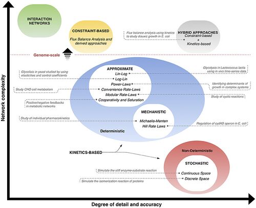Modelling - Figure 1. Comparing different modelling methods according to their accuracy and network complexity Constraint-Based Dynamic Advantages Allows for fast calculations of large networks under the steady state assumption Relies mainly on genetic information easily obtainable by genome sequencing and does not need kinetic data Can model highly dynamic mechanisms such as translational regulation, metabolite concentrations and thermodynamics Reaction kinetics are accounted for Predict and optimize the productivity of a metabolic pathway i.e the rate at which a metabolite is produced, which is important for informing economic viability Disadvantages Model does not take kinetic factors into account Less accurate Only get information about yield (flux) due to the steady state assumption No transient state information Can’t account for regulatory pathways Comprehensive model with many parameters Challenging to model complex organisms Lack of knowledge on many kinetic parameters Modelling - Table 2. Advantages and Disadvantages of constraint based modelling and dynamic modelling When considering which modelling approach to use for modelling we can look at the advantages and disadvantages of both approaches depicted in table 2. There are two main reasons for why dynamic models are much more applicable for cell free systems than constraint-based methods. Firstly, within cells there are homeostasis regulation mechanisms allowing metabolite concentrations to remain relatively constant over time. For cell-free systems these homeostatic regulations do not exist, causing metabolite concentrations to vary over time. As seen in table 1, since constraint-based methods only employ stoichiometric measures, they cannot account for transient behaviors. Thus since it is a stationary modelling method working at the equilibrium point, it assumes metabolite concentrations are constant over time and cannot accurately represent a cell free system. Dynamic modelling can take this into account. The other reason is that in cell free systems, resource competition is an important behaviour, since there are only a fixed amount of resources in the cell free extract. This has to be accounted for in modelling, and constraint based models cannot take this into account. For these reasons dynamic modelling can better represent cell free systems. Parameter Estimation A big challenge for dynamic modelling is the estimation of kinetic parameters. Since many issues arise when using parameters from different sources, parameter estimation techniques are used to find optimal values of parameters. Parameter estimation uses an optimization algorithm that searches through many possible values, under specific constraints and non-linear structures, and then finds complex objective functions with many solutions through local optima. Thus, the goal of optimization problems is to find a global optimum in a reasonable time employing local or global methods. Local methods start the optimization with reference parameters measured or found in literature and then these are improved by each run of the algorithm. These algorithms are often based on the Hessian and gradient of the objective functions, computed numerically through methods like finite difference approximations. Local methods however do not always find the global solution depending on its neighborhood. Global methods use metaheuristics including simulated annealing and genetic or evolutionary algorithms. Combining global and local methods is the most successful method when the solutions are close to an optimal. The most common approach to find the objective function is to minimize the difference between the model output and the experiment data. This approach was used in the dynamic modelling by Wayman et. al and Horvath et. al. Databases and Tools Pathway Databases KEGG – sub databases of genes and proteins, chemical substances, interaction and reaction networks EcoCyc & MetCyc – databases of experimentally illustrated metabolic pathways, Ecocyc specifically for metabolic pathways of E.coli BRENDA – comprehensive enzyme database that allows for an enzyme to be searched by name, EC number or organism Tools for Metabolic Modelling Pathway tools – bioinformatics software package that assists in the construction of pathway/genome databases ERGO - integrates data from every level including genomic, biochemical data, literature, and high-throughput analysis into a comprehensive user-friendly network of metabolic and non-metabolic pathways KEGGtranslator – app that can visualize and convert KEGG files ModelSEED – resource for the analysis, comparison, reconstruction and curation of genome scale metabolic models SCAMP – simulation package Examples Toward a genome scale sequence specific dynamic model of cell-free protein synthesis in Escherichia coli In this study, a dynamic mathematical model of E.coli cell free protein synthesis was developed. CFPS model equations were defined using the hybrid cell-free modelling framework of ‘Wayman et.al’ that integrates kinetic modelling with a logical rule-based description of allosteric regulation. The model parameters were approximated from measurements of glucose, organic acids, energy species, amino acids and the protein product chloramphenicol acetyltransferase (CAT). A constrained Markov Chain Monte Carlo (MCMC) algorithm was employed to estimate a collection of 100 model parameter sets, which minimized the squared difference between model simulations and experimental measurements. A range for each kinetic parameter was established from the BioNumbers database. The constrained MCMC approach estimated parameter sets with a median error 2 times less than using random parameter sets generated from the bounds in literature. The kinetic models were then used to examine the performance of the CFPS system and to find the pathways most important to protein production. The metabolic network was divided into 19 reaction groups and group knockout analysis was used to estimate the effect of different network functions on protein synthesis. It was found that CAT was produced with an efficiency of 12%, which showed that a lot of the energy resources for protein synthesis were channelled to non-productive pathways. By simulating the knockout of metabolic enzyme groups, it was shown that metabolism and protein production were reliant on oxidative phosphorylation and glycolysis/gluconeogenesis. References TX-TL Modelling N.B It should be noted that although primary sources are cited below, much of the general understanding stems from the mini review published by Koch et al., 2018. What is TX-TL? Transcription-Translation (TX-TL) modelling extends the standard model of gene expression to cell-free systems. It takes into account, as its name suggests, the shared transcriptional and translational machinery in in-vitro cell-free systems. Typically, TX-TL models are classified as dynamic, deterministic models and hence involve modelling the kinetics of the cell-free system through non-linear ordinary differential equations. This involves breaking down the process of transcription and translation into two similar equations and relating these to the rate of protein production through various parameters, whilst adhering to the various conservation laws outlined below. Since these models use non-linear ODEs they cannot be solved analytically, parameters must either be measured experimentally or estimated using software. Generally, TX-TL models require few external parameters and those that are required generally have clear physical interpretations meaning most can be quantified experimentally. In the papers reviewed below the model parameters were tuned using parameter tuning software alongside real experimental data. Ideally this is the approach we would take in developing our model, however due to the current COVID-19 situation it is unlikely that we will be able to secure sufficient lab time to gather the in-vitro data. One approach could be to test and tune our model based on data which has already been collected for similar metabolites. Why use TX-TL for Cell-Free Systems? In-vivo modelling techniques are designed with several active cellular processes in mind, in cell-free systems many of these processes no longer continue to run. Additionally, several environmental differences exist for example molecular crowding , the significantly altered resource distribution and the lack of resource competition with the host. It follows that to accurately model a cell-free system these standard modelling techniques must be adapted to take these environmental differences into account. What do TX-TL Models Predict? Cell-free systems are used for protein production, according to the rate of protein production can be broken down into four phases: 1) Increasing rate of production, 2) Constant rate of production, 3) Decreasing rate of production, 4) Rate of production is zero. And for mRNA production: 1) Increasing concentration, 2) Constant concentration, 3) Decreasing concentration, 4) Concentration close to zero. These phases are summarised in TX-TL - Figure 1. 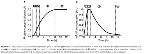TX-TL - Figure 1. From Koch et al., 2018, Summarises the four phases of protein and mRNA production TX-TL models are deterministic models which use ODEs to describe transcription, translation, mRNA and protein degradation processes and fit these to the phases described above using various parameters. The General Assumption The total DNA concentration is constant Usually, a protected linear template or plasmid DNA is inserted into the cell-free system for protein production, since no dNTPs are added replication can be ignored. Since the half life of DNA is so long DNA degradation is generally neglected too. General Issues One issue which is consistently outlined in papers is that batch-to-batch variations in systems can often have a significant impact on how the system behaves. This means that the values of parameters can also vary widely between batches, as well as from in vivo to cell-free. A Basic Model The following model by Karzbrun et al. requires ten parameters and fits the protein and mRNA dynamics described above whilst remaining coarse grained. Parameters were derived based on experiments which used cell extract solely comprising of Escherichia Coli machinery. Transcription Dynamics [math]\displaystyle{ \dot{m}(t) = k_{TX} \cdot N^{-1}_m [R_pD]- \frac{m(t)}{\tau_m}, \forall t \gt \tau_0 }[/math] Translation Dynamics [math]\displaystyle{ \dot{p}_{syn} = k_{TL} \cdot N^{-1}_p \cdot \frac{m(D, t-\tau_f)}{1 + K_{TL}/R} }[/math] Where Rp = RNA Polymerase R = Ribosome Xm = RNAse (RNA degradation enzyme) Xp = Protease (protein degradation enzyme) D = DNA m = mRNA p = protein kTX = Rate of transcription kTL = Rate of translation In this model the transcription rate depends on two factors: the binding rate of RNA polymerase to the DNA and the length of the DNA strand. The authors found that the model was able to accurately predict TX/TL and degradation dynamics for phases 1 and 2, however the model did not reach a steady state. Additionally, the degradation modelled occurred at a constant rate rather than exponentially. This points to the model being appropriate for use in a cell-free system prior to resource consumption or waste accumulation cause the reaction to halt, this is approximately the first 60 minutes. A TX-TL Model Based on Michaelis-Menten Kinetics Stögbauer et al. established a rate equation model with eight free parameters which fit the experimental data they gathered. Experimentally the concentration of GFP present in the reaction mixture was measured using a spectrometer. A cell-free expression system which consisted of reconstituted components was used, the system was RNAse and protease free (neglecting degradation through proteins) and contained 50 purified components. The model builds on using deterministic rate equations to capture transcription and translation, specifically Michaelis-Menten and Hill kinetics were tested. Transcription Dynamics [math]\displaystyle{ \dot{mRNA} = \frac{k_ts \cdot TsR \cdot DNA}{K_s + DNA} - \delta_{mRNA} \cdot mRNA }[/math] Translation Dynamics [math]\displaystyle{ \dot{GFP} = \frac{k_tl \cdot TlR \cdot mRNA}{K_l + mRNA} - k_{mat} \cdot GFP }[/math] [math]\displaystyle{ \dot{GFP}^* = k_mat \cdot GFP }[/math] Prefactors [math]\displaystyle{ \dot{TsR} = - \frac{k_Cs \cdot TsR \cdot DNA}{K_s + DNA} }[/math] [math]\displaystyle{ \dot{TlR} = - \frac{\delta_{TlR} \cdot TlR}{K_{TlR} + TlR} }[/math] Where kts = Rate of transcription ktl = Rate of translation kmat = Rate of protein (GFP) maturation TsR = Transcription resource (consumed by transcription process with scaling factor kcs) TlR = Translation resource (consumed with rate δ TlR independently of the translation process) ks, ki = Michaelis constants The transcription and translation dynamics are represented through Michaelis-Menten like reactions. The authors note that since no proteases were present in the lysate GFP degradation has been ignored, so applying this model to a normal cell-free system would require the addition of a protein degradation term. Models of this type fit the early and late phases of biosynthesis reactions whilst remaining coarse grained (i.e. simple). Variations of TX-TL Models Involving Michaelis-Menten Kinetics Authors have built upon the model above leading to more detailed descriptions of the TX-TL processes. Tuza et al. added reversible binding of RNA Polymerase, a reversible binding of the first amino acid as well as an irreversible elongation step. Similar reversible binding reactions were applied to the translational equation. Moore et al. also developed a model which took the above into account, as well as the sharing of the NTP energy source (i.e. an energy source for cellular reactions). Both models mentioned in this section led to more accurate predictions of cell-free systems due to the additional properties of the cell-free system that they captured. Resource Competition The following resources are limited in a typical cell-free system: NTPs, ribosomes, RNA polymerase, elongation factors, chaperone proteins, tRNA synthase. It follows that in a typical cell-free system the reason for phase 2 (constant rate of protein production) is because of a limitation of at least one of the mentioned resources. The models mentioned below describe competition for fixed amounts of transcriptional and translational resources only, i.e. they do not take into account metabolite production or consumption. TX-TL Models Which Consider Resource Competition Algar, Ellis and Stan produced a model which focuses on translational elongation in chassis cells, assuming that the resources for transcription are far less restricted than those for translation. The model, which is derived from first principles in their paper, is a probabilistic model which uses deterministic nonlinear ordinary differential equations. In a separate paper, some of the same authors tested the existing model in a cell-free system. The paper focussed on using cell-free assay to predict the demands of expressing a protein in Escherichia Coli (in vivo), their findings showed that the in-vitro system could accurately predict the in vivo results. Given the current global situation, this paper suggests that when testing our in-silico model, we can use similar in vivo data as a suitable alternative to gathering in vitro measurements. However, this raises the question that if in vitro models can be tuned using in vivo data from the equivalent system, why can the parameters of the standard model of gene expression not be tuned to suit in vitro systems? Borkowski et al. also found that increasing DNA concentration only increases protein production until a saturation point has been reached. They suggest that this could owe to the higher transcriptional rate using up resources shared between the translation and transcription portions of the system, one such example is GTP. GTP is used as a nucleotide during transcription as well as an energy source when elongation occurs during translation. Gyorgy and Murray proposed a dynamic model which focused on resource competition, namely the limited availability of RNA polymerase and ribosomes. The equations are outlined below: Transcription Dynamics [math]\displaystyle{ b_i + p \underset{k_i^+}{\stackrel{k_i^-}{\rightleftharpoons}} c_i \qquad and \qquad c_i \stackrel{\alpha_i}{\rightarrow} b_i + p + m_i }[/math] Translation Dynamics [math]\displaystyle{ m_i + r \underset{k_i^+}{\stackrel{k_i^-}{\rightleftharpoons}} d_i \qquad and \qquad d_i \stackrel{\alpha_i}{\rightarrow} m_i + r + x_i }[/math] Degradation Dynamics [math]\displaystyle{ m_i \stackrel{\delta_i}{\rightarrow} 0 }[/math] [math]\displaystyle{ d_i \stackrel{\delta_i}{\rightarrow} r }[/math] [math]\displaystyle{ x_i \stackrel{\gamma_i}{\rightarrow} 0 }[/math] Resulting model [math]\displaystyle{ \dot{b}_i = -(k_i^+ pb_i - k_i^-c_i) + \alpha_i c_i, }[/math] [math]\displaystyle{ \dot{c}_i = -(k_i^+ pb_i - k_i^-c_i) - \alpha_i c_i, }[/math] [math]\displaystyle{ \dot{m}_i = \alpha_i c_i - \delta_i m_i - (k_i^+ m_ir - k_i^-d_i) + \beta_i d_i, }[/math] [math]\displaystyle{ \dot{d}_i = (k_i^+ m_ir - k_i^-d_i) - \beta_i d_i - \delta_i d_i, }[/math] [math]\displaystyle{ \dot{x}_i = \beta_i d_i - \gamma_i x_i, }[/math] Where bi = Promoter of protein xi ci = Promoter bound to RNA polymerase mi = Resulting mRNA transcript p = RNA polymerase d = ribosome transcript complex TlR = Translation resource r = ribosome (ribosome transcript complex degradation) δ = rate of protein xi degradation (dilution) This model reaches a quasi-steady state but only through assuming that the rates of protein production and decay are far slower than the rates of the binding and unbinding reactions. The authors also note that this model is only accurate until phase 2 (constant rate of protein production). Metabolism Koch et al. mentions that the approaches discussed above can be less accurate when used on cell-free metabolic engineering systems. This is because the dynamic models do not consider metabolites as part of the limited resources, cell-free metabolic engineering systems (CFME) often compete for metabolites. Constraint-based models are used to predict the metabolic production of the entire CFME system and dynamic models are used for the transcription and translation dynamics of individual proteins. It is important to consider metabolic activity on a system level since each protein can have varying dynamics along the pathway, but the rate of metabolite production is still governed by the rate limiting step. In their review Koch et al. notes that the field of modelling CFME systems is in its infancy and so very few models exist at the moment. They also note that despite these being constraint based models, only a few constraints have been identified, this raises the question of how accurate these models are in general systems. Implementing Models A handful of ‘toolboxes’ have been created by research groups to aid the implementation of models. These contain pre-written functions, usually in MATLAB, which represent each protein in the system . Obtaining Parameter Values Parameters that cannot be measured through experiments must be estimated by using software to fit the parameters of the model to the relevant experimental data. The simplest algorithm is the Random Walk. This takes random steps over a given range of numbers and uses this value for the parameter. The error between the prediction and the experimental data is then measured. This repeats and the algorithm is stopped after a set time and the best parameters are taken. Moore et al. mentions two other methods: Bayesian Statistical Inference and Maximum likelihood point estimates. The first involves treating each parameter as a random variable. This means that each parameter will have a probability density function, these become narrower as more data is added, pointing to the best values. The author states that maximum likelihood point estimates have some shortcomings in complex parameter estimation situations. Model Types Summary Models based on Michaelis-Menten kinetics fit the early and late stages of cell-free systems well. They remain accurate and coarse-grained throughout this. Models which focus on resource competition in cell-free are accurate until phase 2 (constant rate of protein production). These usually only require parameters which can be measured experimentally, and in some cases remove the need for parameter estimation. References Paper Reviews Introduction The aim of this section is to provide a high level overview of papers relating to the project. The views outlined here are purely the interpretation of the group. Quantitative Modelling of Transcription and Translation of an all-E. coli cell-free system Introduction TXTL: simple coarse grained descriptions that capture a CFPS system’s basic mechanisms in a single set of equations Pros: can report on saturation of the TXTL components Cons: limitations of the system are not considered / are missing Working principles: linear & saturation response regimes of gene expression wrt... Plasmid concentration Strengths of the regulatory parts ie. promotor, sigma factor Concentration of TXTL machinery Different TXTL platforms/ models: PURE system Integrates only highly purified components within a test tube to facilitate in vitro protein synthesis. Extract-based system Cell-free lysate containing relevant substrates (ie. amino acids, ATP, nucleotide) and machinery (ie. regulatory factors, enzymes) Cell system used in paper: Conventional T7 hybrid TXTL. Bacteriophage transcription, T7 RNA polymerase and promoter, is coupled to the translation machinery of E. coli. TXTL systems’ broad TX repertoires allow for testing of many regulatory elements with different strengths, as opposed to the T7 hybrid systems. This refers to promoter and UTR are from T7 phages The synthesis of whole phages (ie.T7 and T4) demonstrates that an all-E. coli TXTL system’s endogenous TX machinery can process large DNA programs containing tens of regulatory elements with strengths spanning several orders of magnitude. Outcome of paper: simple non-stochastic ODE model of an all-E. coli TXTL system Suitable for CFPS performed in batch mode in microliters scale & in well-mixed reactions Model is tested with and applied to a set of 3 promoters specific to the primary sigma factor 70 (rpoD) in combination with a set of 3 untranslated regions. Both spanning a strength of about two orders of magnitude. Rates of protein synthesis determined in the steady state for 9 combinations wrt (1) plasmid concentrations and (2) TXTL components concentrations. Robustness of the model tested against several key biochemical constants experimentally determined to constrain the model fitting and simulations. The model captures the major TXTL regimes and saturations, which are predominantly due to the depletion of ribosomes on the mRNAs. The synthetic and natural E. coli sets of regulatory parts are compared. To establish a reference table of the performances of regulatory elements between TXTL and in vivo. Goals for a good model: Accessible: can be interpreted, understood and used by other people Facilitate tuning, setting of component concentrations Choosing of strengths and stoichiometry of regulatory parts making circuits TX: Transcription Ktx, the initiation frequency for transcription depends on kcat,m, KM,70, and E70. kcat,m is the rate constant for mRNA synthesis, KM,70 is the michaelis Menten constant, E70 is the complexed core RNA polymerase with sigma factor 70 Ktx has a max of 30 initiations per 60 seconds. This limits kcat,m to 0.5(1/s) kcat,m was estimated to be between 0.1 and 0.001(1/s) for E.coli promoters. For a strong promoter it is expected that kcat,m is at the high end of these estimations. In the best fit kcat,m was estimated to be 0.065 (1/s) KM,70 is typically between 1nm and 100nm. KM,70 was estimated to be 1nm from the best fit. The total concentration core RNA polymerases in E.coli varies between 1500 and 11400 molecules per cell, depending on growth conditions. The lysate for the TXTL system is prepared from cells growing in a rich medium and *collected in the exponential phase, so the concentration of core RNA polymerase is at the high end of 11000-12000 per cell. The maximal concentration of core RNA polymerase is estimated to be around 1.5um if all the *enzymes are released during preparation, which translates to a maximum of Etot = 500nM of core RNA polymerase in the TXTL reaction.The minimum concentration of free core RNA polymerase is found by only considering the *polymerases not bound to DNA, the best fit was Etot = 400nm. To calculate the sigma factor 70: there are 500-700 copies per cell. In the TXTL reaction, sigma 70 is at a maximum concentration of about 30-35nm and that fits the best fit. K70 = 0.26 is the dissociation constant between sigma 70 and the core RNA polymerase The rate constant of the deGFP mRNA degradation is determined by assay: 1/Kdeg,m = 0.000825s.This constant is written as Kdeg,m = kd,m/KM,m. kd,m = 6.6nM/s and KM,m =8000nM. The concentration of promoter P70 and gene is determined experimentally The length of the transcribed gene is Lm = 750 bp , from the transcription start to the terminator The average speed of transcription is estimated by an assay Cm = 10bp/s Calculating the mRNA steady state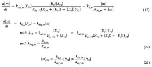 The mRNA steady state is found by setting equation 17 equal to zero. For low plasmid concentrations (in the linear regime), one can assume that E70>>KM,70. This results in the term [E70]/(KM,70 +[E70]) being approximately one and we can therefore approximate KTX ~ Kcat,m TX machinery is never limiting the system because the rate of mRNA synthesis keeps increasing even at plasmid concentrations larger than 5nM. TL machinery is that that limits the system - ribosomes are entirely depleted onto the mRNA at plasmid concentrations above 5nM TL: Translation The following section contains a summary of the translation part of this TXTL system; the parameters, how they were measured/estimated/determined and the derived equations. kTL: initiation frequency for translation, depends on both kcat, p and KM,R, as well as R0; similar to transcription; kTL can be as high as 0.5 s-1. KM,R: The MM-constant for translation was measured in vitro to be around 23 nM for the 70S ribosome with no tRNA and 10 nM with tRNA. In a previous cell-free system, KM,R was fitted at 65.8 nM. Here, KM,R = 10 nM was used for the best fit. kcat, p: rate constant of protein synthesis. No estimation of kcat, p was found in literature. For low mRNA concentrations, one can expect that R0 >> KM,R, putting a limit on kcat, p to 0.5 s-1. kmat: rate constant for maturation of deGFP. Determined by an assay described in previous work. [R0]: concentration of free ribosomes. The avg. concentration of ribosomes in E.coli cells growing in a rich medium, with a doubling time of 20-30 minutes, is between 44000-73000 nM, which corresponds to 1450-2500 nM in a TXTL reaction. This is in agreement w.r.t. previous measurements in cell-free systems. [Rtot] : total concentration of active ribosomes in TXTL. Rtot = 1100 nM was best fit for active ribosomes in TXTL. Average translation speed (speed of ribosomes on mRNA): estimated to be at least 1 amino acid per second (2.5 bp/s) Rate of deGFPdark production: 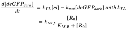Steady state for deGFPdark: 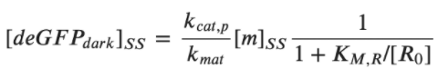For low plasmid concentrations [P70] < 1 nM, one can expect KM, R/R0 << 1. Hence, we get: 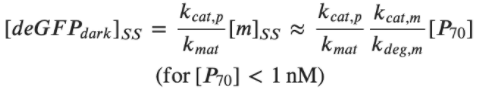A simple expression for the linear accumulation of deGFPmat at low plasmid concentrations is then: 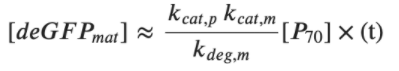At 1 nM plasmid P70a-deGFP, we measure a maximum protein synthesis rate of 0.5 nM/s, which indicates that the product kcat,p*kcat,m = 4 10−4 s−2 (taking kdeg,m = 8.25 10−4 s−1 for the deGFP mRNA) The value for kcat,p = 6 10−3 s−1 was chosen based on this calculation using kcat,m = 6.5 10−2 s−1. A maximum theoretical value (1 nM plasmid ≈ 1 copy per E. coli) of 300 nM/s for the protein synthesis rate in TXTL is obtained by taking kcat,m ≈ kcat,p = 0.5 s−1 and a 1/kdeg,m ≈ 20 min. As shown in the paper for plasmid P70a-deGFP concentrations of 1, 5 and 10 nM, the model delivers reliable kinetics at SS for the first few hours, below and above the transition from linear to saturated regimes A hallmark of Noireaux’s approach is how the model accurately grasps the sharpness between the linear and saturated regime (see Figure 2 in the paper) Another model (https://doi.org/10.1093/nar/gkt052) describing similar TXTL system, based on a different regeneration system, attributes the translation saturation to metabolic processes and energy efficiency – though when applied to P70a-deGFP, this approach neither captures the linear regime nor the sharpness of the response observed in this work The authors assume that the behaviour of cell-free expression (e.g. presence of a linear response regime and the sharpness of the transition from linear to saturated) in both models (systems) do not have the same origin Parts Combination and Sensitivity Analysis Two promoters and two UTRs, P70b and P70c and UTR2 and UTR3 are derived from P70a and UTR1 respectively. The -35 and -10 of P70a were mutated to get P70b and P70c and the ribosome binding site in UTR1 was mutated to get UTR2 and UTR3. kcat, p,kcat,m and the Michaelis-Menten constants KM,70 (transcription) and KM,R (translation) are changed due to the change in promoter and UTR strengths kcat, p: rate constant of protein synthesis kcat,m : the rate constant for mRNA synthesis Because the system is only weakly sensitive to changes in magnitude of the Michaelis-Menten constants, they were not changed in the TXTL model The rates of protein synthesis for the 9 combinations were experimentally determined with respect to plasmid concentration The sensitivity analysis comprised of varying each of the 6 biochemical constants and keeping all others constants at their best numerical fit values P70a-UTR1- translation is the limiting process responsible for saturation of protein synthesis rate as plasmid concentration is increased But as seen in the plots, for weak promoters, the protein synthesis rate is linear for any plasmid concentration (up to 30 nm) kdeg,m : If kdeg,m is larger, the system doesn’t saturate and the response remains lower but if kdeg,m is smaller, then the system saturates more quickly with respect to plasmid concentration. Rtot: model and data most sensitive to ribosome concentration, especially for strong promoter but for weak promoter, it’s not as obvious Etot: saturation not observed in experiments, limitations due to Etot only observed if #0 <100 nm KM,70, KM,R: weak sensitivity S70: model not sensitive Strengths of synthetic vs natural regulatory elements Chose constitutive promoter of genes, some based on protein abundance and isolated by coupling them to a strong UTR1: lacI, rpoH, rrsB, recA. Chose UTR of genes by coupling each of them to strong promoter P70a. Defined rates of deGFP synthesis per plasmid concentration (deGFP/h/nM) for each construction in linear regime as an indication of both promoter strength and UTR strength. This quick method of TXTL can be used to test many other promoters and UTRs TXTL load calculator Determine burden on TXTL components, especially translation machinery Developed equation taking into account promoter strength, UTR strength, length of gene being expressed in DNA construct to create model predictions fo the approximate limiting DNA concentration for different promoter strengths, UTR strengths and lengths of genes Running the model derived in this paper using the group's own code The commented code for this paper can be found in the following Google Colab Notebook: https://colab.research.google.com/drive/1FfpIHa75qd5xZmYeDokivv2ZSVVmwu21?usp=sharing Version 1 The group was advised to follow the industry standard of TX-TL simulation and code the model using Python. Google Collaboratory was used to enable several group members easily to work on the same code in a Jupyter Notebook style document. In the first version of the code (Noireaux(V1).ipynb) a function was written to calculate constants E0 (concentration of free RNAP), R0 (concentration of free ribosomes) and mSS the mRNA concentrations at the steady state. The naming convention used was “calc_” followed by the name of the constant. It was often necessary to solve an equation which was set equal to zero to obtain the value of these constants, to do this the solveset function from the sympy library was used. It was necessary to isolate the positive real roots following the use of the solveset function. The three ODEs (equations 17, 18 and 19) in the paper were modelled using a function representing the 3-equation system (function model) and the function was solved (function txtl) using the odeint function from the scipy library. A second ODE system was added to the model (functions degrad_model and degrad_txtl), in which a linear degradation term was added to equation 19. This meant that the concentration of deGFPmat no longer increased infinitely. This system of equations was also solved using the odeint function. The matplotlib library was used to plot the various graphs found in the paper. Comparisons of the group’s code and the figures from the Noireaux paper can be found in the figures below: Whilst the code captures the correct shape of the relevant figures in the paper, the values predicted by the code are not correct. Version 2 of the code will address this. We have confirmed that the graphs in the paper are indeed experimental data and not from the TXTL model Version 2, 3 and 4 In later versions of the code, a parameter vector was used for clarity. This included all the previously used parameters. The ODEs were rewritten into sums of linear rates, where each rate represents a different chemical reaction. Sensitivity analysis was also added by incorporating parameters for P70b and its corresponding UTR2 and P70c and corresponding UTR3. General code readability improvements were also carried out: including more functions and comprehensions. Five different functions were created to compute the concentrations: E0, R0, Mss and deGFPss. A further new function was created to modify the parameters corresponding to the chosen promoter, which changes the kcat,m and kcat,p values in the parameter vector. Finally, a new parameter was added to the TXTL model to incorporate degradation in the sum of linear rates.
Recently Edited Notebook Pages 2020-12-05 07:12:52 User:VisvaM/Notebook/Applications of Cell-Free Protein Synthesis and Biosensors to Metabolic Engineering/Entry Base 2020-11-22 11:25:12 User:VisvaM/Notebook/Applications of Cell-Free Protein Synthesis and Biosensors to Metabolic Engineering/Entry Base