Computational Methods for The Millikan Oil Drop Experiment

^{SJK 00:15, 29 November 2009 (EST)}

00:15, 29 November 2009 (EST)
Overall, this is a very good rough draft. Most of the things here are excellent, so the primary issues are missing items. Some of the missing things are quite substantial, especially in the methods and results sections, as you can see from my comments. But I think you'll be able to fill those in very well and produce a really great final draft. For the "extra data," I do want you to try to get some more droplets, and it'd be good if there were some closer to 1, 2, etc. charges. Also for "extra data," I think fitting Millikan's data as well as using simulated data (as you and I discuss below) would be a really good thing.

Contact Information

Author: John J. Callow

Experimentalists: John J. Callow & Johnny Gonzalez

Location: University of New Mexico Physics and Astronomy Department, Albuquerque, NM

e-mail: jcallow@unm.edu

Abstract

^{SJK 17:41, 28 November 2009 (EST)}

17:41, 28 November 2009 (EST)
It is customary to use the past tense for reporting results. So, in your first two sentences, you should say, e.g., "We observed the behavior of several oil droplets ..." "The oil droplets were produced...". Later, I would also say, "...an integer multiple of the value of e, we developed an algorithm... (again past tense). Also, abstracts are typically space-constrained, so you wouldn't have the line breaks that you do, but would rather report the numbers in-line in the text. Other than these style issues, I like your abstract. It is notable that you do not motivate the experiment (electron charge is important, because...), nor do you give future implications. So it's outside the kind of framework I presented. But that's OK, because I think it coherently presents an abstract of your study, assuming a bit of knowledge by the reader. That's OK with me. I think you need to clearly define what "e" represents, though: "charge (e)".

In this experiment we will observe the behavior of several oil droplets in a uniform electric field to find each droplets individual charge, and then using statistical methods calculate the charge of a single electron. The oil droplets will be produced by an atomizer, allowed to settle between two parallel plates acting as a capacitor, and then viewed with a telescope. By comparing the time for a droplet to fall a specified distance with no field to the time that same droplet takes to rise up that distance with an electric field applied we are able to calculate the mass of the drop and then find the charge. Using the assumption that electrons are identical and there is no fractional charge, each charge observed must be some integer n times the value of e, and then using a developed algorithm for the problem a value for e is found that best matches these assumptions.

Our value for the charge of a single electron is

[math]\displaystyle{ e = 4.839(20)*10^{-10} e.s.u. }[/math]

The value found from Millikan

[math]\displaystyle{ e = 4.774(9)*10^{-10} e.s.u. }[/math] [2, pg 140]

The currently accepted value is

[math]\displaystyle{ e = 4.803*10^{-10} e.s.u. }[/math]

Both our and Mullikan's are very close to the currently accepted value and thus showing that this experiment is very effective even compared to modern methods such as (fill this in later) for finding the charge of a single electron.

Introduction

^{SJK 22:14, 28 November 2009 (EST)}

From the results of J J Thomson's charge to mass ratio experiment concrete proof was finally available that the electron existed.[read this article] That different materials all had the same result in Thomson's experiment gave good reason to believe that all electrons carried the same charge. Soon Thomson would begin experiments to determine e, one of which was observing a cloud of identical water droplets carrying a single charge and the effects of gravity or an electric field on said cloud where observed.[1]. But because of the uncertain rate of evaporation and that there was no way to verify each drop was identical and carried a single charge, this method had high uncertainty in its experimental values.

Soon Millikan came up with his oil drop experiment, which eliminated most of the uncertainty of previous experiments. Also unlike the water cloud, Millikan's experiment allowed for the direct observation of a small number of charges on a single oil drop, giving further evidence that electrons are all identical. One issue with Millikan's experiment is that its accuracy greatly depended on Stokes's law and the assumption that oil droplets would behave as solid spheres. After a correction was introduced to Stokes's law for drops approaching the size of the mean free path of a gas molecule, and performing the experiment with liquids of varying viscosity, Millikan found they all produced the same result within error tolerance. Thus the assumption that the drops behaved as solids was shown to introduce little error and so was valid [2, pg 111]. Since the major issues with the experiment had been resolved, Millikan eventually found that e = 4.774(9)*10^-10 e.s.u. [2, pg 140] which is very close to the modern accepted value of 4.803*10^-10 e.s.u.[source]. That an experiment about one hundred years old holds up so well to modern methods demonstrates just how ingenious it is.

In our experiment we reproduced Millikan's original, observing individual charged oil drops in gravity alone and in an electric field. The reasoning for doing the report is to not only verify Millikan's findings being how important they are to atomic physics, but to also experimentally test an algorithm designed to solve under-determined systems of equations by restricting variables to a specified set of numbers. In our case, we are restricting each [math]\displaystyle{ {n_i} }[/math] to solve the system of equations [math]\displaystyle{ {n_i}*e = {q_i} }[/math] for the charge of an electron e where each q is the total charge found on each drop. Though methods have already been developed to solve for e using data from this type of experiment, it is hard to pass up the chance to explore others as understanding in physics or any science is commonly tied to mathematical concepts.

Methods and Materials

Taking Data

^{SJK 22:33, 28 November 2009 (EST)}

22:33, 28 November 2009 (EST)
Title of this section isn't the typical parts of speech used (I think that's the correct terminology). Something like "data acquisition" is more typical.

Now that I've read further, I notice that what you have here is essentially a description of the apparatus (that is a good thing), but missing entirely is methods for data collection. So, you should probably rename this section "commercial Millikan oil droplet apparatus" or something like that (also including a photo or diagram would be very good as Figure 1). Then you need to add a section, something like "measurement of droplet rise and fall times." You'll include information about how the apparatus was focused. How was oil sprayed. How were times measured. (e.g., "One experimenter (JG) selected a droplet which seemed to have approximately __ fall time. JG called out "start" and "stop" and these times were recorded by the other experimenter (JC) using [web applet or whatever stopwatch(reference)]). You can skimp on some of the details, that you think are less important, but I'd link to those as a reference. You can make the reference something like "3. Full methods can be found at [link]"

We used a commercial Millikan oil drop apparatus kit (pasco something) which consisted of a telescope, capacitor, oil droplet housing, light source, thermistor, and atomizer. Oil sprayed from the atomizer into the housing was viewed from the telescope. A switch allowed for us to turn off and on an electric field caused by the capacitor plates and an external power supply(tel-atomic 500V DC supply). A grid built into the telescope allowed us to accurately observe the rise and fall times over .5mm of an oil drop.

To correctly apply Stokes's law, we needed the temperature in the chamber along with the barometric pressure. To keep track of the temperature a multimeter was connected to the apperatus's thermistor. With this reading, the temperature can be found that corresponds measured resistance to temperature. Due to lack of time we used the initial reading of the thermistor finding the temperature to be 27 degrees centigrade [4]. We estimated the barometric pressure to be 76.0 cm of mercury using a reading done at the time at a nearby airport [3]. Because we didn't have exact values for either temperature or barometric pressure, this introduced minor error.^{SJK 22:18, 28 November 2009 (EST)}

22:18, 28 November 2009 (EST)
Both of these would be obvious things to improve when you retake data. Also, I'd like you to investigate whether the pressure you get from the weather report is the actual pressure, or whether it's been adjusted to sea level.

To calculate the charge of an electron from these times we needed to observe several drops of different charge. The apparatus had the ability to ionize droplets using a radioactive thorium 240somethins source exposed by a lever. This allowed for us to view a single sized drop with different charges. Because electrons have negligible mass compared to a drop of oil, this proved to be a great method as the fall times remained the same. It also insures that the data collected is that of drops with different charge which is required by our algorithm to find e.

Analysis

^{SJK 23:19, 28 November 2009 (EST)}

23:19, 28 November 2009 (EST)
I think absolutely you should describe your fitting algorithm in the methods (as opposed to only in an appendix). It is a key part of your report, especially since it's innovative. Even if it weren't innovative, it's critical to the final answers you get, so it needs to be described in main part of paper at least a little. You don't need to include the full code (linking to that is fine), but you should write out the formula, and describe in words w/ formula how it works. I think that's quite do-able. Also, if you know of any similar procedure in math or experimental science, by you should by all means point that out and include citations. Given that you should expand the analysis section, I think what you have now should be renamed "calculation of droplet charge." The next section could be named "algorithm for finding most likely value of elementary charge."

With the data collected we were able to calculate the charge on each individual drop by using the formula

[math]\displaystyle{ q = \left[400{\pi}d\left(\frac{1}{g{\rho}}{\left[\frac{9*{\eta}}{2}\right]^3}\right)^{\frac{1}{2}}\right]*\left[\left(\frac{1}{1+\frac{b}{pa}}\right)^{\frac{3}{2}}\right]*\left[\frac{V_f+V_r\sqrt {V_f}}{V}\right] e.s.u. }[/math]

in which q is the charge of the drop, d the separation of the capacitor plates, [math]\displaystyle{ {\rho} }[/math] the density of oil, g the acceleration of gravity, [math]\displaystyle{ {\eta} }[/math]-viscosity of air in poise, b a constant equal to [math]\displaystyle{ 6.17*10^{-4} }[/math] cm of Hg, p the barometric pressure, a the radius of a drop, and V the potential difference across the plates. Then plugging the values for each charge into an algorithm written in Matlab 7.1.0 we were able to find the charge of an electron. This algorithm may be found in the appendix along with info on the above formula and constants.

Tables and Figures

^{SJK 22:43, 28 November 2009 (EST)}

22:43, 28 November 2009 (EST)
Tables need numbering and captions, just like figures. Even if you have only one, it'd be "Table 1"

^{SJK 23:02, 28 November 2009 (EST)}

23:02, 28 November 2009 (EST)
Since it's fairly easy to embed these images as thumbnails, I think it's better to put them close to the section of text where you talk about the figures. This makes it easier for the reader. When you submit a paper to many journals for peer review, you in fact still have to separate figures and legends from the rest of the text. But that's just a legacy issue that hopefully will go away someday.

^{SJK 23:09, 28 November 2009 (EST)}

23:09, 28 November 2009 (EST)
For figures 2 and 3, I think you should have a name for the y-axis, rather than "see below." Something like "net euclidean distance" or "goodness of fit" or something that you want to call it. Figure 1 is close to being a completely good caption. It's good that you specify red versus blue dots. However, it's still a bit of a challenge for reader to determine what's going on. You can specify in legend exactly what x-axes is: calculated charge, and y-axis: charge divided by e. Now that I think about it, why aren't there x-error bars? Also, I'm a bit confused now, too: I like how it demonstrates the difference between integer charges with the red versus blue. However, isn't this plot guaranteed to be linear no matter what the data are?

After making my comments elsewhere, I can now say this about your figures overall: They are very good (some improvements can be made as noted), but you will undoubtedly need to present more results as either more figures and / or more plots overlayed on these figures.

Droplet	Rise Time seconds	Fall Time seconds	Rise Velocity cm/s	Fall Velocity cm/s	Charge 10^-9 e.s.u.
1	4.18(8)	17.34(40)	0.0120(2)	0.0029(1)	4.74(17)
2	3.49(4)	9.34(14)	0.0143(2)	0.0054(1)	9.17(17)
3	1.31(8)	11.56(47)	0.0387(25)	0.0044(2)	9.74(46)
4	6.23(30)	11.70(24)	0.0081(4)	0.0043(1)	6.74(17)
5	2.82(14)	16.9(1)	0.0179(10)	0.0030(1)	5.35(19)
6	5.65(14)	13.66(25)	0.0089(2)	0.0037(1)	5.83(16)

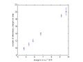Figure 1: A plot with the error bars around the calculated values of each drop divided by my algorithms best estimate of the charge of an electron as blue dots and the closest integer value times the charge of an electron as red dots.
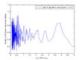Figure 2: Plot of the output of the function used in my algorithm. The graph represents charge e vs. the euclidean distance between each droplets charge q/e and its rounded value. The minimum of this value is our best estimate for the charge of an electron.
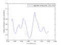Figure 3: A close up view around the minimum.

Results and Discussion

^{SJK 23:28, 28 November 2009 (EST)}

23:28, 28 November 2009 (EST)
This section will have to be expanded quite a bit. There are two reasons for this. (A) The first is that you are not providing enough explanation and discussion for what you're already presenting. (B) The next reason is that I think you should include more results in your final draft. As far as (A) goes, here's an example of what's missing. You should start out the results by describing Table 1! The first main result is really your calculation of the droplet charges, along with the uncertainty. So, you should present that first. "We collected rise and fall times for __ droplets. __ of these were discarded due to problems of ___. This left 6 droplet charge measurements for 5 distinct droplets (one droplet was successfully ionized as shown in rows __ and __ of Table 1. etc.

Next, you want to talk about how you apply your algorithm to find the most likely value of elementary charges. At this point you'll really need to describe what the figures mean, and what assumptions are made (e.g., what range of possible values? do you assume that you have less than 100 charges on each, etc.?)

I have a really hard time describing the difference between results and discussion, and that's why I tend to group the two sections. Results are supposed to be more matter of fact (this is what the charges are) whereas discussion is supposed to be more interpretive and putting forth assertions requiring more questionable modeling or requiring more assumptions. I'll be happy to talk with you more about this. OK, as for (B), I really think you have a lot more results you can show: first of all, you'll have more data in a couple weeks. More than that, though, it is very much worth showing how your algorithm performs with Millikan's data. Plus, you can look at that LabVIEW application I linked for you and you could either use it or Matlab to simulate droplet charges and explore how robust your algorithm is. You may not have time for rigorous results, but you could indicate things like "how much noise can be tolerated? what causes algorithm to fail? etc." These new things will naturally produce more figures. Or you could group similar figures (such as your function plotted for Millikan's and your data overlayed)

Figure 2 shows a plot of our algorithm trying to find the best value for the charge of an electron numerically using values from .1 to 5*10^-9 e.s.u. The method is based on finding a minimum euclidean distance between two vectors, where each value is q/e in one vector and this value rounded to the nearest whole number in another. As shown in the plot, the minimum appears at just about 4.8*10^-10 e.s.u. This function begins to oscillate wildly as e->0 simply because q/e is being evaluated. Figure 3 shows a window from 4.8-5*10^-10 e.s.u. giving a better view of how the function is behaving on a smaller scale.

In Figure 1 I plotted the charge divided by our best estimate of e for all the drops in blue with error bars and the closest integer multiple of our estimated e as red dots. From the plot it is clear that not only does each red dot lie well within the error bars but that they lie nearly on top of the calculated charges of the drops. This gives a lot of confidence in our method for finding e, and also tells us that the data we took is likely very accurate. All except one drop had very small standard error, and even our worst drop had standard error that is less than our best estimate for e.

Conclusions

^{SJK 23:32, 28 November 2009 (EST)}

23:32, 28 November 2009 (EST)
The middle of this paragraph (talking about number of steps) is more like a result / discussion. I think missing from the conclusion is a statement that you developed an algorithm (maybe novel?) that can be applied to this experiment and perhaps others.

Because we were unable to aquire exact values for the air pressure and forgot to record the thermistor reading for each individual measurement a bit of error is introduced here, but likely very little. Though accuracy in measuring rise and fall times alone had appriciable error, because of the power of the developed algorithm we still found a very good approximation for the charge of an electron. Our value for e was [math]\displaystyle{ e = 4.839(4)*10^{-10} e.s.u. }[/math] using 1,000,000 steps in the algorithm. Even with only 1000 steps though it estimates e at [math]\displaystyle{ e = 4.871(4)*10^{-10} e.s.u. }[/math], and this is with a very generous interval over which the algorithm searches. The uncertainty was calculated using a similar method to that of linear regression. Compared to the accepted value of [math]\displaystyle{ e = 4.803*10^{-10} e.s.u. }[/math] we differ by less than .5%. Though with current data our standard error doesn't overlap the accepted value, with improved measurements and better values for air pressure and temperature it is very likely they will.

With both or results and that of Millikan's being so close to modern methods of experimentally finding an electron's charge, it really shows how powerful this method is for being fairly simple to set up. Being able to observe the effect of only a few charge also gives us very strong visual evidence that electrons are all equivalent.

Acknowledgments

I would like to thank my lab partner Johnny Gonzalez for helping with setting up and taking data in this experiment. Also I thank my professor Dr. Koch and assistant Pranav Rathi for answering questions and assisting with some setup.

References

[1] Modern Physics fifth edition, Paul A. Tipler and Ralph A. llewellyn

[2] Millikan R.A (1913), On the Elementary Electrical Charge and the Avogadro Constant. Physical Review, 2 pp. 109-143

[3] http://www.widespread.com/daily.aspx?id=2580&d=10%2f21%2f2009 (it seems to have broken since originally doing the lab)

[4] Pasco Millikan Apparatus lab manual http://openwetware.org/images/e/ea/Pasco_millikan_manual.pdf

To be added

I'd like to have a section under analysis on experimenting with the algorithm if I'm unable to actually prove anything. This would be things such as using simulated data and having it attempt to find some value.^{SJK 23:33, 28 November 2009 (EST)}

23:33, 28 November 2009 (EST)
I saw this statement after making my comments above...I agree!!! I really love the idea of using simulated data (adding in noise and / or systematic error) to explore the robustness of your algorithm.

Appendix

^{SJK 23:38, 28 November 2009 (EST)}

23:38, 28 November 2009 (EST)
It is very good that you're providing your code, please do keep doing that. However, as noted above, you should also describe the algorithms in the methods section. I already discussed how you should explain your euclidean distance fit parameter in the methods. You should also describe the uncertainty. Since I can't read maple files, I have no idea what you're doing...so I can't evaluate it. It seems strange that your uncertainty is so small, especially since you can get two distinct values for different step sizes with error bars that don't overlap with each other. That makes me wonder whether you're underestimating your uncertainty. Another way you could estimate your uncertainty is to use simulated data. First, you find your best fit value and assign integers to each droplet. Then, you use random numbers to generate 6 (or however many) new charge values with new random noise of same size as your original droplets. Fit the random data to find e_1. Then repeat this 100 or 1000 times to find the spread in the e_n values.
As for formal proofs, I think that'd be really cool, but I'm OK if you save that for when you have time for more open-ended problems.

Here is where I plan on putting more info on how the algorithm works, and how I calculate it's uncertainty. I derived a method for it's uncertainty based off that of linear regression but not sure if this is anywhere near what should be done. Also analysis of my function has me believing that the value it puts out is provable to be the best estimate on a reasonable interval. I'll see if I can manage proof in time to turn in the final draft but it might be a bit beyond my current abilities given the time and that I don't really know much statistics other than what I've learned in this class. If I can't do some formal proofs though the experiments would probably be convincing enough.

Matlab Code

Algorithm used to find an electron's charge

Error propagation code

Maple Worksheets

Worksheet used to calculate error for each droplet's charge

Raw Data from Lab Notebook

{{#widget:Google Spreadsheet |key=teM0-yaHA6q25ObiMTpXVyQ |width=650 |height=450 }} {{#widget:Google Spreadsheet |key=tFvCtsSivUGACvsbaBisHzQ |width=650 |height=450 }} {{#widget:Google Spreadsheet |key=tobGh-FK6kkY1qNgzuRjiwQ |width=650 |height=450 }} {{#widget:Google Spreadsheet |key=tPeiQVkSGPOmNGPO9EotBUw |width=650 |height=450 }}

List of Used Constants and Their Values

[math]\displaystyle{ {\rho} }[/math] - density of oil [math]\displaystyle{ \frac{.866g}{cm^3} }[/math]

g-acceleration of gravity [math]\displaystyle{ \frac{981cm}{s^2} }[/math]

b-constant equal to [math]\displaystyle{ 6.17*10^{-4} }[/math] cm of Hg

V-potential difference across the plates 500 volts

p-barometric pressure 76.0cm of mercury found at http://www.widespread.com/daily.aspx?id=2580&d=10%2f21%2f2009. Used value at time 15:56 as that is around when measurements took place. Unfortunately the pressure inside the lab is probably different, but we had no equipment to measure it.^{SJK 22:57, 28 November 2009 (EST)}

22:57, 28 November 2009 (EST)
http://www.wunderground.com is another site for archived values. Is pressure indoors really that much different? It doesn't seem very windy when doors are opened. Also note question above: is the air pressure actual or is it corrected to sea level?

Formulas

[math]\displaystyle{ q = \left[400{\pi}d\left(\frac{1}{g{\rho}}{\left[\frac{9*{\eta}}{2}\right]^3}\right)^{\frac{1}{2}}\right]*\left[\left(\frac{1}{1+\frac{b}{pa}}\right)^{\frac{3}{2}}\right]*\left[\frac{V_f+V_r\sqrt {V_f}}{V}\right] e.s.u. }[/math]

[math]\displaystyle{ a = \sqrt {\left(\frac{b}{2p}\right)^2 + \frac{9{\eta}*V_f}{2g{\rho}}}- \left(\frac{b}{2p}\right) }[/math]

User:John Callow/Notebook/Junior Lab/Formal Report

Contents