User:John Callow/Notebook/Junior Lab/Final Formal Report
Computational Methods for The Millikan Oil Drop Experiment
Contact Information
Author: John J. Callow
Experimentalists: John J. Callow & Johnny Gonzalez
Location: University of New Mexico Physics and Astronomy Department, Albuquerque, NM
e-mail: jcallow@unm.edu
Abstract
In this experiment we had two goals, first to repeat Millikan's Nobel prize winning oil drop experiment, and second find the fundamental charge of a single electron e using an algorithm based off Euclidean distance in an N dimensional space developed by us to fit the data. An accurate value of e being used in not just physical experiments, but chemistry, biology, and all sorts of engineering fields. Although this experiment is the only current use of the algorithm, we find it important to test and develop so that in similar cases where one must extract a value that divides a given set of data evenly this method may be added to the current tools of solving these problems. Using these methods, we find [math]\displaystyle{ e = 4.839+/-.3*10^{-10} e.s.u. }[/math], which is in agreement with both the modern value of [math]\displaystyle{ e = 4.803*10^{-10} e.s.u. }[/math]5 and Millikan's original value of [math]\displaystyle{ e = 4.774(9)*10^{-10} e.s.u. }[/math] 2.
Introduction
From the results of J J Thomson's charge to mass ratio experiment concrete proof was finally available that the electron existed.6 That different materials all had the same result in Thomson's experiment gave good reason to believe that all electrons carried the same charge.1 Soon after Thomson began experiments to determine e, one of which was observing a cloud of identical water droplets carrying a single charge and the effects of gravity or an electric field on said cloud where observed.1 But because of the uncertain rate of evaporation and that there was no way to verify each drop was identical and carried a single charge, this method had high uncertainty in its experimental values.
Soon Millikan came up with his oil drop experiment, which eliminated most of the uncertainty of previous experiments. Also unlike the water cloud, Millikan's experiment allowed for the direct observation of a small number of charges on a single oil drop, giving further evidence that electrons are all identical. One issue with Millikan's experiment is that its accuracy greatly depended on Stokes's law and the assumption that oil droplets would behave as solid spheres. After a correction was introduced to Stokes's law for drops approaching the size of the mean free path of a gas molecule, and performing the experiment with liquids of varying viscosity, Millikan found they all produced the same result within error tolerance. Thus the assumption that the drops behaved as solids was shown to introduce little error and so was valid.2 Since the major issues with the experiment had been resolved, Millikan eventually found that e = 4.774(9)*10^-10 e.s.u. 2 which is very close to the modern accepted value of 4.803*10^-10 e.s.u.5. That an experiment about one hundred years old holds up so well to modern methods demonstrates just how ingenious it is.
In our experiment we reproduced Millikan's original, observing individual charged oil drops in gravity alone and in an electric field. The reasoning for doing the report is to not only verify Millikan's findings being how important they are to atomic physics, but to also experimentally test an algorithm designed to solve under-determined systems of equations by restricting variables to a specified set of numbers. In our case, we are restricting each [math]\displaystyle{ {n_i} }[/math] to solve the system of equations [math]\displaystyle{ {n_i}*e = {q_i} }[/math] for the charge of an electron e where each q is the total charge found on each drop. Though methods have already been developed to solve for e using data from this type of experiment, it is hard to pass up the chance to explore others as understanding in physics or any science is commonly tied to mathematical concepts.
Methods and Materials
Commercial Millikan oil droplet apparatus
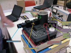
We used the commercial Millikan oil drop apparatus AP-8210 kit shown in Figure 1 which consisted of a telescope, capacitor, oil droplet housing, light source, thermistor, and atomizer. Oil sprayed from the atomizer into the housing was viewed from the telescope. A switch allowed for us to turn off and on an electric field caused by the capacitor plates and an external power supply(tel-atomic 500V DC supply). A grid built into the telescope allowed us to accurately observe the rise and fall times over .5mm of an oil drop.
To correctly apply Stokes's law, we needed the temperature in the chamber along with the barometric pressure. To keep track of the temperature a multimeter was connected to the apparatus's thermistor. With this reading, the temperature can be found that corresponds measured resistance to temperature. Due to lack of time we used the initial reading of the thermistor finding the temperature to be 27 degrees centigrade 4. We estimated the barometric pressure to be 76.0 cm of mercury using a reading done at the time at a nearby airport 3. Because we didn't have exact values for either temperature or barometric pressure, this introduced minor error.
Measurement of droplet rise and fall times
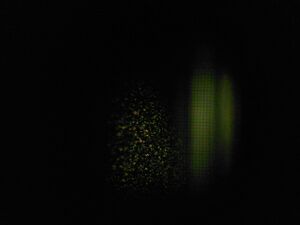
We viewed the droplets through a telescope that was focused using a wire from the apparatus placed in the viewing chamber. With the telescope focused, we then sprayed oil into the viewing chamber using an atomizer. After a few minutes the majority of droplets fell out of view leaving only a few left to choose from. By doing this we greatly reduced the chance of either losing sight of a chosen drop or that there would be nearby interference from other droplets. When choosing a drop to track, we observed the rate at which the drop fell with no electric field and then the rate it rised with a 500V field. By choosing drops that behaved differently each time this made sure our data was of drops of different charges which by our methods was required to find e. Figure 2 shows a photo of the droplets inside the chamber.
Once a drop was chosen one experimentor would track a drop while the other managed the stopwatch. The tracker called out to start timing when the drop was crossing a viewable major gridline and then call out stop once it had passed the next major gridline. This was repeated several times with field on and off for each droplet viewed. For more detailed information on setup and taking data see http://openwetware.org/wiki/User:John_Callow/Notebook/Junior_Lab_307/2009/10/14#Setup.
Analysis
Calculation of Droplet Charge
With the data collected we were able to calculate the charge on each individual drop by using the formula
[math]\displaystyle{ q = \left[400{\pi}d\left(\frac{1}{g{\rho}}{\left[\frac{9*{\eta}}{2}\right]^3}\right)^{\frac{1}{2}}\right]*\left[\left(\frac{1}{1+\frac{b}{pa}}\right)^{\frac{3}{2}}\right]*\left[\frac{V_f+V_r\sqrt {V_f}}{V}\right] e.s.u. }[/math]
in which q is the charge of the drop, d the separation of the capacitor plates, [math]\displaystyle{ {\rho} }[/math] the density of oil, g the acceleration of gravity, [math]\displaystyle{ {\eta} }[/math]-viscosity of air in poise, b a constant equal to [math]\displaystyle{ 6.17*10^{-4} }[/math] cm of Hg, p the barometric pressure, a the radius of a drop, and V the potential difference across the plates.2
Algorithm for finding most likely value of elementary charge
To find the value of an elementary charge we developed a formula based off the distance between a point and the origin of an N dimensional Euclidean space7 where
[math]\displaystyle{ distance = {(\sum_{n=0}^N x_n^2)^{.5}} }[/math].
Using each charge divided by a suspected value of e and then subtracting from this the same value but rounded to the nearest integer as coordinates for a point in a N dimensional space we have that
elementary charge = [math]\displaystyle{ e \in I }[/math] such that [math]\displaystyle{ (\sum_{n=0}^N {(\frac{q_n}{e}-round(\frac{q_n}{e}))^2}) }[/math] is minimized,
where N is the number of different charges, each q_n is the charge of one of our droplets, and I is the interval that the value of the fundamental charge is suspected to be in. To find this minimum, we used a script written in Matlab 7.1.0 that may be found in the Matlab Code section of the appendix.
The idea behind the method is to find a value such that it goes into each droplet charge found as close to an integer value as possible. If it is assumed that there is no fractional charge, then this value is very likely to either be the best value given a set of data for the elementary charge, or at least is some multiple of it. To rule out whether it is just a multiple either the plot of the data must be examined to check other nearby minimums found. If the issue of having several best values for e is apparent, currently the only method to rule out other values is by gathering more data and eliminating values that divide all data points evenly. As the set of data becomes increasingly large, the chance of not finding a droplet with an odd charge becomes small which validates the elimination of these minimums. Another method for ruling out multiples of the minimum is to shrink the interval I by assuming the value must be close to that found in other experiments that attempt to find the same value, or finding other assumptions likely to be true that may be applied.
Results and Discussion
Results from Our Experiment
Table 1
| Droplet | Rise Time seconds | Fall Time seconds | Rise Velocity cm/s | Fall Velocity cm/s | Charge 10^-9 e.s.u. |
|---|---|---|---|---|---|
| 1 | 4.18(8) | 17.34(40) | 0.0120(2) | 0.0029(1) | 4.74(17) |
| 2 | 3.49(4) | 9.34(14) | 0.0143(2) | 0.0054(1) | 9.17(17) |
| 3 | 1.31(8) | 11.56(47) | 0.0387(25) | 0.0044(2) | 9.74(46) |
| 4 | 6.23(30) | 11.70(24) | 0.0081(4) | 0.0043(1) | 6.74(17) |
| 5 | 2.82(14) | 16.9(1) | 0.0179(10) | 0.0030(1) | 5.35(19) |
| 6 | 5.65(14) | 13.66(25) | 0.0089(2) | 0.0037(1) | 5.83(16) |
Data gathered during our experiment.
Table 1 displays the rise and fall times for each of the 6 trials of taking data along with the calculated charge. Trials 3 and 4 are the same droplet but with 4 being measurements taken after ionizing the droplet. As seen in the table, the uncertainty in the fall times of the two trials overlap which is clear evidence that changing the charge does very little to change the mass of a droplet. The other 4 droplets were unique giving us a total of 5 different droplets observed. For the complete set of data which includes several measurements of rise and fall times for each drop see the appendix.
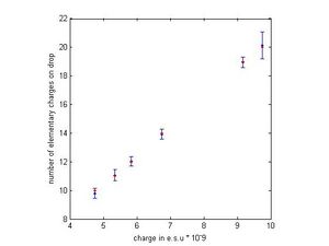
In Figure 3 the plot shows the charge divided by our best estimate of e for all the drops in blue with error bars and the closest integer multiple of our estimated e as red dots. From the plot it is clear that not only does each red dot lie well within the error bars but that they lie nearly on top of the calculated charges of the drops. This gives a lot of confidence in our method for finding e, and also tells us that the data we took is likely very accurate. All except one drop had very small standard error, and even our worst drop had standard error that is less than our best estimate for e. As will be shown in the next section the algorithm will completely break if the noise level is too high in the data.
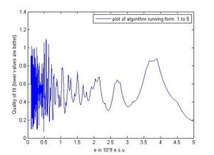
Figure 4 shows a plot of our algorithm trying to find the best value for the charge of an electron numerically using values from (.1 to 5) where a single unite represents 10^-9 e.s.u. The number of steps was set to 100,000 for the plot. We chose this interval based on a few assumptions. If the fundamental charge happens to be much less than .1, the accuracy of our experiment has almost no chance of finding it. This is because our data is only accurate out to two decimal places, so a number this small either is too far under our estimated uncertainty or once reaching a certain point it begins to divide any possible data point evenly. For example, .01 goes into all of our data exactly, but if the fundamental charge is this small our methods aren't valid for finding it. Also seen from the plot, the function begins to behave very wildly around this point which is caused by the fact that a as e becomes smaller, the amount e must be changed to go into the calculated droplet charges also becomes very small.
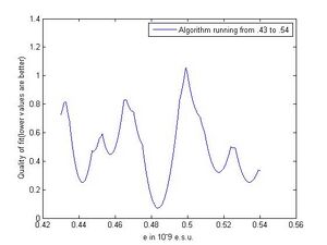
The reasoning for stopping at 5 is we make the assumption that no partial charge was observed, and with our smallest data point being 4.74 running the algorithm much past that point would mean if a minimum was found beyond this range, the value the algorithm found would imply we found partial charge. Figure 5 shows a window from .48-.5 giving a better view of how the function is behaving on a smaller scale. If by some other experiment or reasoning the interval I could be assumed to be small such as this, this figure also demonstrates that the function is much better behaved on small intervals and that the minimum is much more defined. So if at all possible it is best to force the interval I to be small to achieve best results. We did not take enough data to rule out much though, and though we could have used other previous experimental results other than ours to shrink the interval we tried to use as few assumptions as possible. However if our result was far off from other experiments, we would have had to done something along those lines to pull the correct minimum from the algorithm.
Using the algorithm with our collected data we found [math]\displaystyle{ e = 4.839+/-.3*10^{-10} e.s.u. }[/math] which is about 0.7% off the modern accepted value of [math]\displaystyle{ e = 4.803*10^{-10} e.s.u. }[/math]. The average uncertainty in the droplet calculations is about 3-4% so using figure 6 we expect the algorithm to return values that deviate by 6% which is about [math]\displaystyle{ {+/-}0.3*10^{-10} e.s.u }[/math]. This is not a 66% confidence interval, but instead is closer to 100%. Our 66% confidence interval should be much smaller considering the points in figure 6 are much denser around 0.48. Even with that in mind though, it is still very likely that the accepted value differs by less than one standard error of the mean so our experiment was in agreement with modern experiments.
For find the uncertainty a better method is to take a sufficiently small interval around the calculated point and then approximate the distance formula by regular functions. On small intervals there is very likely to be an exact formula not involving a round function and using that it would be possible to calculate uncertainty in the usually matter of taking a derivative at the point with respect to the coordinate variable, multiply by uncertainty of the charge and square the value, sum over all the coordinates, then take the square root. This is a bit beyond the scope of this report though, so I only give this brief outline given the possibility anyone wishes to further develop these methods.
Using Simulated Data To Test The Limits of Our Algorithm
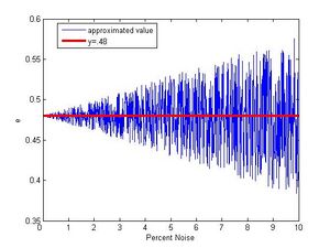
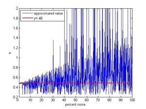
To find just how accurate we may expect our fitting function to be we use simulated data. The data is created by taking a random value from one to twenty, multiplying it by .48(the actual value) and then adding noise by multiplying this value by 1 + the percent noise.(Steve Koch 12:42, 14 December 2009 (EST):How many simulated drops did you use?) Figure 6 shows a plot of 1000 trials with noise ranging from 0 to 10%. For small noise the function does a very good job approximating e. Even as noise grows the densest area of this plot still tends towards the correct value. Figure 7 shows simulated data with noise ranging from 0 to 100% and up till about 15% the function will give back the appropriate value. Beyond that even though the pattern of gradually growing outwards from .48 is visible, the behavior of the function begins to become more erratic with nonsense values popping up. Also viewable in Figure 7 is the function sometimes picking the half value. As pointed out in the analysis section, with enough droplets it is possible to statistically rule this out and then being left with the full value as the best estimate again. The code used to make these plots was developed in matlab 7.1.0 and may be found in the appendix.
This simulated data gives a fairly reliable way to decide whether this type of algorithm is applicable to a given set of data. Our uncertainties were small thus our suspected noise is small. That the algorithm gave back the correct value strengthens that this approach to noise estimation works. If the uncertainty in a set of data is relatively large so is the noise, so using this algorithm is likely not the best approach. Even with bad data one could try to shorten the interval I and possibly find the correct minimum. Given the nature of the function, it isn't difficult to find a minimum of the function around what is expected, so it is however necessary to have good reason to shorten interval I.
Conclusions
Both our results ([math]\displaystyle{ e = 4.839+/-.3*10^{-10} e.s.u. }[/math]) and Millikan's ([math]\displaystyle{ e = 4.774(9)*10^{-10} e.s.u. }[/math]) are very close to the modern accepted value of the elementary charge ([math]\displaystyle{ e = 4.803*10^{-10} e.s.u. }[/math]). Considering the technology available during the time of this experiment these results show just how powerful and clever the oil drop experiment is. In addition to being a very accurate method, it allows and experimentor to clearly see the effects of only a few elementary charges acting on a droplet of oil. With these observations it is clear that in general there is easily observable half charge, and if such charges ever exist in nature at all after taking a sufficient number of data points the experiment shows that this is a very rare occurrence (Steve Koch 12:45, 14 December 2009 (EST):I'm not sure what you're saying here. Do you mean that you definitely have the precision to detect half-charges, if they exist?).
The algorithm method developed for this experiment has shown to be very accurate when the noise level of the data is reasonable. Though complete reasoning for why this method works and it's limitations is beyond the scope of this paper, the experiments using simulated data shows clear evidence that there is some validity to its results. Perhaps with formal proof the method could be modified to better approximate e based on uncertainty in data by changing the metric from being based off Euclidean to another metric. But even with the results and ideas here, the algorithm could easily be modified for other uses involving the approximation of an underlying constant value that shows up in multiples of itself in data. One such example could be the Balmar series, and likely there could be applications found in signal processing. And even if there is little use outside this experiment, it is always worth investigating ideas in mathematics as there is bound to be further uses in the future.
Acknowledgments
I would like to thank my lab partner Johnny Gonzalez for helping with setting up and taking data in this experiment. Also I thank my professor Dr. Koch and assistant Pranav Rathi for answering questions and assisting with some setup.
References
[1] Modern Physics fifth edition, Paul A. Tipler and Ralph A. llewellyn
[2] Millikan R.A , "On the Elementary Electrical Charge and the Avogadro Constant." Physical Review, 2 pp. 109-143 (1913)
[3] http://www.widespread.com/daily.aspx?id=2580&d=10%2f21%2f2009
[4] Pasco Millikan Apparatus lab manual http://openwetware.org/images/e/ea/Pasco_millikan_manual.pdf
[5] Handbook of Chemistry and Physics 82nd Edition 2001-2002, David R. Lide
[6] J. Thompson, "Cathode Rays". The London, Edinburgh, and Dublin Philosophical Magazine and Journal of Science, Vol 44, 293-316 (1897)
[7] Introduction To Topology second edition, Theodore W. Gamelin and Robert Everist Greene
Appendix
Matlab Code
Algorithm used to find an electron's charge
Noise generating and plotting code
Maple Worksheets
Worksheet used to calculate error for each droplet's charge
Raw Data from Lab Notebook
List of Used Constants and Their Values
[math]\displaystyle{ {\rho} }[/math] - density of oil [math]\displaystyle{ \frac{.866g}{cm^3} }[/math]
g-acceleration of gravity [math]\displaystyle{ \frac{981cm}{s^2} }[/math]