User:Cristhian Carrillo/Notebook/Physics 307L/2010/11/10

e/m Ratio

• Please note that Ginny was my lab partner for this lab.

Purpose

The purpose of this lab is to measure the charge-to-mass ratio of the electron by studying the effects of electric and magnetic fields on a charged particle.

Equipment

Total Apparatus

(bottom) Hewlett-Packard DC Power Supply (Model 6384A, 4-5.5V, 0-8A) and (top) BK PRECISION Digital Multimeter (Model 2831B, SER. NO. 000-03-0618 , 5 WATTS, 8 VA,50~60 Hz)

e/m Experimental Apparatus (Model TG-13)

(left of e/m E. A.) SOAR corporation DC Power Supply (Model 7403, 0-36V, 3A), (top right) BK PRECISION Digital Multimeter (Model 2831B, SER. NO. 099-10-0357 , 5 WATTS, 8 VA,50~60 Hz), (bottom right) Gelman Instrument Company Deluxe Regulated Power Supply (500 V, 100 mA)

measuring scale

image of electron beam

• Hewlett Packard DC Power Supply (Model 6384A, 4-5.5V, 0-8A)
• e/m experimental apparatus (Model TG-13)
• SOAR corporation DC Power Supply (Model 7403, 0-36V, 3A)
• Gelman Instrument Company Deluxe Regulated Power Supply (500V, 100mA)
• 2 BK Precision Digital Multimeter (Model 2831B)

Safety

• Make sure to ground all power supplies properly before use
• Check cords, cables and machinery for any possible electrocution points on fuses of cords
• Protective grounding conductor must be connected to ground
• Be careful with the mercury tube

Setup

We followed the descriptions in Professor Gold's manual and Alex Andrego's Notebook for the setup.

Below are the steps we followed to setup the experiment

• We first used BNC cables to conncect a regulated 6-9V DC supply rated at 2A to the Helmholtz Coil jacks.
• Connected the ammeter in series between the supply and the coil jacks.
• We connected the 6.3V power supply rated at 1.5 A to the heater jacks of the electron gun.
• Connected a high voltage source at 150-300V DC rated at 40mA to the electrode jacks of the electron gun

• Please note that the voltage determines the average velocity of the electron in the beam.

• We then connected the DC voltmeter at the jacks labeled "voltmeter" on the base panel.
• Be sure to turn the current adjust control to zero and set the switch on the panel to the e/m position.

• Make sure that nothing is connected to the jacks labeled "Deflection Plates" at this time.

• Allowed the electron gun filament to heat up for a few minutes after we turned on the heater supply.
• We then applied a 200V DC potential from the high voltage supply to the electrodes.
• Then we turned off the light to begin the experiment.
• Make sure that a black cloth to cover the tube and to backdrop the beam while observing the beam of electrons.
• We then adjusted the current control until the beam formed a circle by turning on the coil current and increasing the current adjustment control.
• We then used the scale behind the bulb to measure the radius of the loop of the beam.

Calculations and Analysis

Below is our raw data {{#widget:Google Spreadsheet |key=0AqzpS6URre5adEVENnRPMkZHTXpKeWVDM2o4V242WUE |width=800 |height=500 }}

• The following equations were used to calculate the e/m ratio.

We found the Helmholtz configuration from Professor Gold's Manual to be:

[math]\displaystyle{ x=R/2\,\! }[/math], [math]\displaystyle{ N=130\,\! }[/math], and [math]\displaystyle{ R=0.15 m\,\! }[/math]

The permeability of free space is given as

[math]\displaystyle{ \mu=4\pi\times10^{-7}\frac{weber}{amp-meter}\,\! }[/math]

From these values we can calculate:

[math]\displaystyle{ B=\frac{\mu R^2NI}{(R^2+x^2)^{3/2}}\,\! }[/math]

We know that the energy of the electron is equal to the kinetic energy:

[math]\displaystyle{ {e}{V}=\frac{1}{2}{m}{v}^{2}\,\! }[/math]

The magnetic force for a charge is...

[math]\displaystyle{ {F}_{B}={q}{v}{B}\,\! }[/math]

The centripetal force is...

[math]\displaystyle{ {F}_{c}={m}\frac{v^2}{r}\,\! }[/math]

Finally we set the centripetal force equal to the magnetic force and obtained:

[math]\displaystyle{ \frac{e}{m}=\frac{{2}{V}}{{r}^{2}}\frac{{(R^2+x^2)}^{3}}{{({u}{R}^{2}{N}{I})}^{2}}\,\! }[/math]

According to Professor Gold's manual, the current accepted value of [math]\displaystyle{ \frac{e}{m}\,\! }[/math] is:

[math]\displaystyle{ \frac{e}{m}=1.76\times10^{11}\frac{C}{kg}\,\! }[/math]

Below is the average and SEM that we found using the above equation [math]\displaystyle{ \frac{e}{m} }[/math] we obtained when we set the centripetal force equal to the magnetic force.

• Average

[math]\displaystyle{ \frac{e}{m}=1.54\times10^{11}\frac{C}{kg} }[/math]

• SEM

[math]\displaystyle{ \frac{e}{m}=2.62\times10^{9}\frac{C}{kg} }[/math]

• Percent Error

[math]\displaystyle{ \% error=12.4%\,\! }[/math]

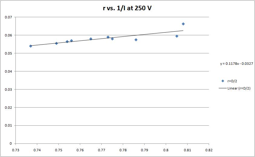
The other way to find [math]\displaystyle{ \frac{e}{m}\,\! }[/math] is to plot

1. [math]\displaystyle{ r\,\! }[/math] vs. [math]\displaystyle{ {I}^{-1}\,\! }[/math], where [math]\displaystyle{ V\,\! }[/math] is constant.

1. [math]\displaystyle{ {r}^{2}\,\! }[/math] vs. [math]\displaystyle{ V\,\! }[/math], where [math]\displaystyle{ I\,\! }[/math] is constant.

From this graph we have that:

[math]\displaystyle{ slope=0.000002\frac{m^2}{V}\,\! }[/math]

We also have that the equation of slope is:

[math]\displaystyle{ slope=\frac{2}{({7.8\times10^{-4}{I})}^{2}}\times\frac{m}{e}\,\! }[/math]

Therefore we can calculate the ratio of [math]\displaystyle{ \frac{e}{m}\,\! }[/math] by:

[math]\displaystyle{ slope=0.000002\frac{m^2}{V}=\frac{2}{({7.8\times10^{-4}{I})}^{2}}\times\frac{m}{e}\,\! }[/math]

[math]\displaystyle{ \frac{e}{m}=\frac{2}{0.000002\times({7.8\times10^{-4}{I})}^{2}}\,\! }[/math]

Where,

[math]\displaystyle{ I=1.324 A\,\! }[/math]

So we have:

[math]\displaystyle{ \frac{e}{m}=\frac{2}{0.000002\times({7.8\times10^{-4}\times{1.324})}^{2}}\,\! }[/math]

[math]\displaystyle{ \simeq9.376\times10^{11}\frac{C}{kg}\,\! }[/math]

Discussion on Error

Reasons for our systematic error

• We had to measure the radius of the electron beam by eye using a fixed ruler in the back of the apparatus. This was hard because we had to roughly estimate for each of the measurements.
• Looking at the second graph above, we can clearly see that there was a larger error for the ratio than the first graph.
• Percent Error for the second graph

[math]\displaystyle{ \% error=\frac{R_{accepted}-R_{measured}}{R_{accepted}} }[/math]

[math]\displaystyle{ \% error\approx4.33%\,\! }[/math]

• This percent error came out better than I thought it would be, so I assume that the error for the first graph would have been even smaller.

Acknowledgements

• I would like to thank Ginny for the great help with this lab and all the other labs we have worked on.
• I would like to thank Katie for helping us with the setup.
• Alex Andrego and Anastasia Ierides for the great pictures and setup instructions.