Roberto Sebastian Rosales/Notebook/Physics 307L/2010/11/10
Steve Koch 21:59, 21 December 2010 (EST): Good primary notebook. You probably had the PMT voltage too low, which would explain your overall very low level of counts. Because of this, you missed, probably, the fact that the Poisson distribution becomes approximately Normal as expected number of counts gets large.
Equipment
- Combined Scintillator and PMT
- Computer running UCS 30 software
- Lead Bricks
- Spectech Universal Computer Spectrometer Power Supply
Safety
There were not any major safety concerns for this lab. When we attempted to collect data a few times, the computer did warn about too high of a voltage for the equipment to handle, so to protect the equipment, we used the voltage as 1000V.
Setup
We followed the setup instructions found in Prof. Gold's Lab Manual. We really only needed to setup the software for the settings that we needed. The scintillator-PMT was already in place in the lead bricks, as well as hooked up to the power supply. This setup was also already connected to the computer. We did find out on the first trial that the UCS 30 software needed to be started after the power supply. If done in the reverse order, the software will show an error notifying that there is no device connected (and quit out on its own I believe).
Procedure
The procedure for this lab consisted of turning on the power supply, starting the software, configuring the software, and finally initiating the counting for each time interval. At first, Matt and I had a little trouble configuring the software, but after a little exploring and some help from Dan, we were able to figure it out. First off, we changed the time interval under the MCS button under Settings (this is where we changed from 10ms to 20ms, from 20ms to 40ms and so on). Then we changed the voltage to 1000V and number of bins to 256 in the main settings menu. We also chose the MCS setting instead of the PHA setting like other groups have done. We double checked Gold's lab manual and it instructed us to use MCS mode. Also, the lab manual said to use the 256 channel setting which is what gave us our 256 bins. For each trial, we simply had to change the Dwell time in the MCS settings, and leave everything else alone.
Data and Calculations
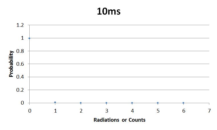
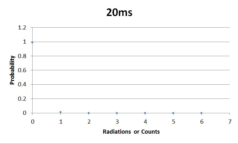
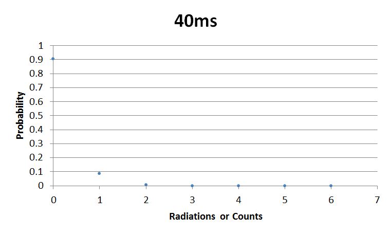
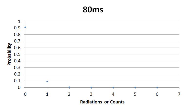
- To collect data, we simply had to initiate the counting process by hitting the green start button. Then I saved the .csv and imported them into Google Docs. The raw data can be found in the spreadsheets below as well as the calculations that I did.
- I took the average in the standard way using:
[math]\displaystyle{ \bar x = \frac{\sum_{i=1} x_i}{n} }[/math], where [math]\displaystyle{ x_i }[/math].
- I found the standard deviation using the built in function in Google Docs, but the real formula is:
[math]\displaystyle{ SD = \sqrt{\frac{1}{N} \sum_{i=k}^N (x_k - mean)^2}. }[/math]
- For the comparison, I found the % error between the standard deviation and the square root of the mean using:
[math]\displaystyle{ % Error = \frac{|x_{calculated} - x_{actual}|}{x_{actual}}*100 }[/math]
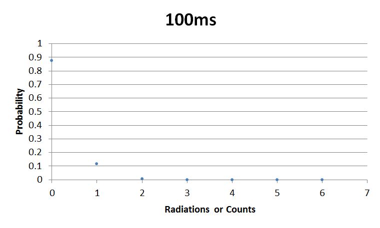
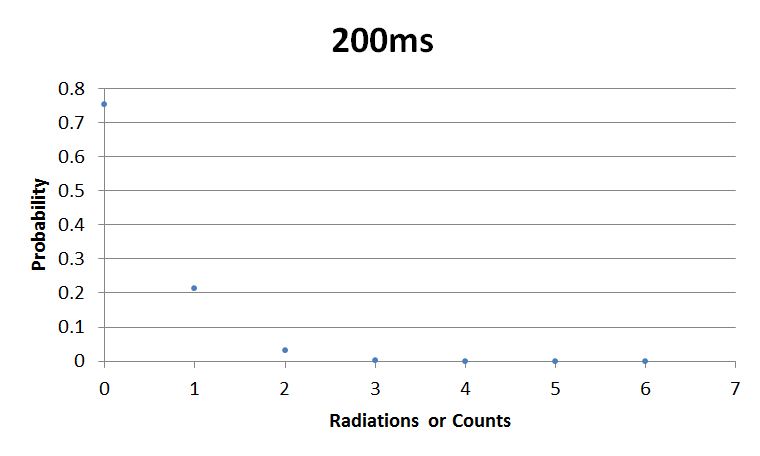
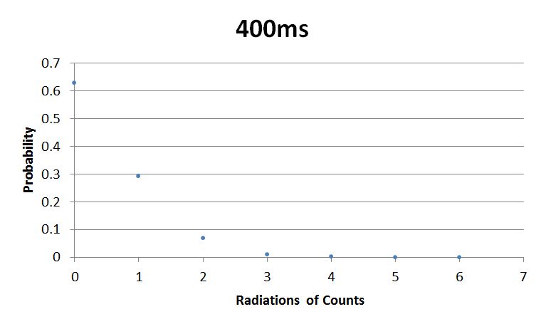
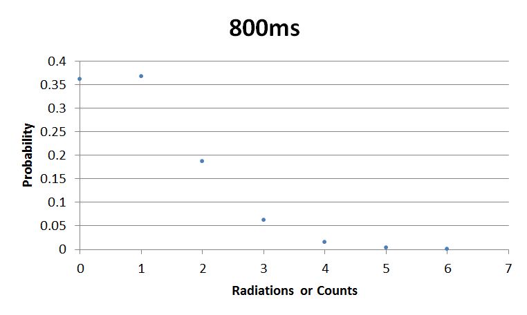
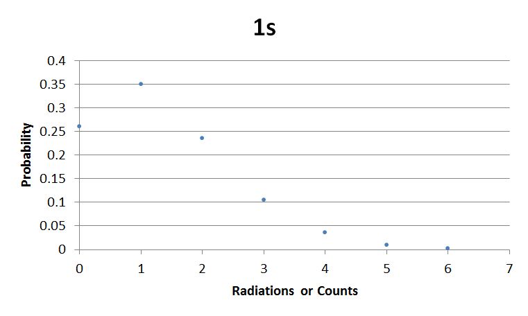
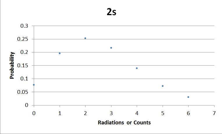
- To find the probability I used the following probability function:
"[math]\displaystyle{ P_\mu (\nu) = e^{-\mu} \frac {\mu^{\nu}} {\nu !} }[/math]
Where:
- P is the probability of ν counts in any definite interval,
- μ is the expected mean number of counts, and
- ν is the number of counts in the interval." - taken from Brian Josey's Lab Summary for Poisson Distribution.
Data
- 10msError in widget Google Spreadsheet: Unable to load template 'wiki:Google Spreadsheet'
- 20msError in widget Google Spreadsheet: Unable to load template 'wiki:Google Spreadsheet'
- 40msError in widget Google Spreadsheet: Unable to load template 'wiki:Google Spreadsheet'
- 80msError in widget Google Spreadsheet: Unable to load template 'wiki:Google Spreadsheet'
- 100msError in widget Google Spreadsheet: Unable to load template 'wiki:Google Spreadsheet'
- 200msError in widget Google Spreadsheet: Unable to load template 'wiki:Google Spreadsheet'
- 400msError in widget Google Spreadsheet: Unable to load template 'wiki:Google Spreadsheet'
- 800msError in widget Google Spreadsheet: Unable to load template 'wiki:Google Spreadsheet'
- 1msError in widget Google Spreadsheet: Unable to load template 'wiki:Google Spreadsheet'
- 2msError in widget Google Spreadsheet: Unable to load template 'wiki:Google Spreadsheet'
References
I used Brian Josey's method for analyzing the data. Instead of graphing wells or bins vs counts, I graphed probability vs counts. Also, Dan W. for assisting us in our initial run through of this lab.
