RAVE:fragility:fragility:input step2generatemodel

Generating the Adjacency Array and Fragility Matrix

Step 2 on the left-hand side is to generate the Adjacency Array. This is the time-varying linear model of the EEG data that will be used to determine the neural fragility of each electrode in the patient. It is generated by using a least-squares algorithm to linearly fit the raw EEG data. The time-varying aspect of this linear model comes from the fact that the entire time course is split into many smaller time windows, and a separate model is generated for each time window. The adjacency array generation process can be thought of as a "sliding time window" process, where the first time window model is generated before "sliding" over by a certain time step and moving on to the next time window.

Clicking the "Generate Adjacency Array" button will load a pop-up with more information on the data you are about to process. Warning: this is the most computationally intensive step and may take a long time (many hours or even multiple days!) to run. This is because a new model is generated for each time window, and there are usually hundreds of time windows. Once the process is finished, a [SubjectCode]_adj_info_trial_# file will appear in your patient's module_data folder. This file will also be loaded for each analysis, so there is no need to generate the adjacency array again unless a different-sized time window or time step is required.

After the adjacency array for a trial has been generated, clicking the "Generate Fragility Matrix" button will calculate the neural fragility values of each electrode over time and generate a [SubjectCode]_f_info_trial_# in your patient's module_data folder. This file is used to create the figures and outputs on the right side of the UI.

In each case, once the files are generated and saved in the module_data folder, there is no need to generate them again unless different parameters are desired. Thus, even though the data processing may be time-consuming at first, it only needs to be done once for each EEG recording.

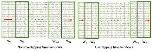
• Timestep explanation: This refers to how far the "sliding time window" moves with each iteration; in other words, whether you want the sequential time windows to overlap or not. If the time step size is equal to the time window size, sequential time windows will not overlap. If the time step size is half of the time window size, each time window will be offset from the previous one by half a time window. Having overlapped time windows results in a more accurate model but slower processing times. See the figure below for an illustration of this concept.