RAVE:CML Workshop 2021

Reproducible Analysis and Visualization of iEEG RAVE

• Home
• Install
• Update
• Launching
• Tutorials and Help
• Community

All steps assume you've properly installed RAVE. All code should be run in RStudio console (or copied into a script and run from there).

Update RAVE to the latest version

Changes were made to facilitate the demo. Even if you just installed RAVE, you must update.

 rave::check_dependencies(nightly=TRUE)
 raveio:::finalize_installation()

If you encounter the following warning:

Warning message:
In i.p(...) :
  installation of package '/var/folders/.../rave_1.0.2.1.tar.gz' had non-zero exit status

Please run

remotes::install_github("beauchamplab/raveio")

followed by

 rave::check_dependencies(nightly=TRUE)
 raveio:::finalize_installation()

Ensure demo data are downloaded

This step may take a while depending on connection speed. Two subjects (and some group data that we won't be using) will be downloaded: KC (~1.1 GB) and YAB (~1.4 GB).

rave::download_sample_data()

Load up the first subject

1. Launch RAVE

rave::start_rave()

2. Project/Subject

Here we want Project: demo and Subject: KC. The first time you select a new subject, you may see a notification (bottom-right of window) saying "Importing AAA", this means RAVE is caching the cortical surface model for subject AAA. This cannot be canceled, but only happens once.

3. Epoch Selection

Choose KCaOutlier for epoch table. For this experiment, 1s Pre and 2s Post event onset is sufficient. Hover your mouse cursor on the Pre/Post input boxes for graphical depiction of timing rules.

4. Electrode & Reference

The default reference table (a common average reference) is the only option. By default, all 10 electrodes are selected. If you accidentally change this, just type in `1-100` to restore the selection.

5. Load Estimation

We're expecting 197 trials, 16 frequencies, 301 timepoints, and 10 electrodes.

6. Load Data!

Power Explorer

After pressing Load Data, RAVE checks the reference file, then defaults you to the Reference Electrodes module. Don't click Load Data. Instead, on the left-hand side, choose Condition Explorer then Power Explorer (Phase Explorer and Voltage Explorer are current in development. Stay Tuned!). Now, the pop up says you need to load Power (Referenced, 156.5 MB). Choose Load Data

There are lots of ways to customize the analysis and graphics options. Explore them! In this tutorial we're going through a pre-set path for time sake. But please, explore!

If you want more horizontal screen real estate, hide the Modules sidebar by clicking "Modules" (grid icon) in the purple bar at the top of the window.

Setting analysis parameters

• Select Electrodes
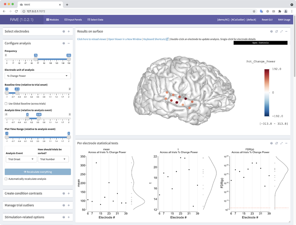
  Keep the default (all electrodes loaded). You can hide this panel by clicking the '-' in the top-right.
• Configure Analysis
  1. Frequency: 72-152
  2. Unit of analysis: Pick your favorite
  3. Baseline time: -1 to -0.5
  4. Analysis time: 0 to 0.55
  5. Recalculate Everything

RAVE is calculating average activity across all trial types. Take a look at the results displayed on the cortical surface model. Click an electrode for information about the electrode. Explore the 3dViewer by selecting "Open Controls" in the top-right of the "Results on surface" panel.

Create a statistical contrast

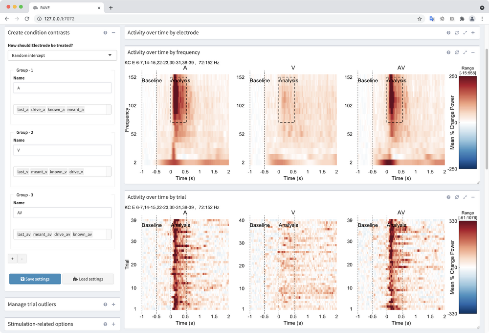
Having visualized the average activity, let's compare the critical conditions in this experiment. In this experiment, we showed participants movie clips of one-syllable words (drive, known, last, meant). The clips were presented either audiovisually (*_av), audio-alone (*_a), or video-alone (*_v).

• Open the "Create condition contrasts" input panel by clicking the "+"
  By default, the first group is named "All Conditions" and has, appropriately, all the conditions.
• Create 3 condition groupings
  Experimental conditions are created in RAVE by assigning trial types to named groups.
  1. A: drive_a, known_a, last_a, known_a
  2. V: drive_v, known_v, last_v, known_v
  3. AV: drive_av, known_av, last_av, known_av
• Save settings
  All analysis settings will be saved to a .yaml file inside your RAVE directory for later use on this or another subject.
• Go back to "Configure Analysis" and click "Recalculate Everything"
  (not required if you earlier had checked the box "Automatically recalculate analysis"

Now that we've created a contrast, scroll to the bottom and take a look at all the graphs. Minimize graphs you don't need by clicking the "-" in the top-right of each output panel. Some graphs may have text that runs out the plot window. You can click the expanding arrows to maximize a given plot.

Copy plots to PowerPoint

RAVE graphs are quite customizable. Checkout the "Configure plots" input panel and explore some of the options. Some of our favorites include playing with the "Lines color palette", the "Heatmap color palette" or setting "Plot background color " to emulate dark mode. Once you have a plot setup, you can copy it directly into PowerPoint.

nota bene. You can control the width of RAVE plots by resizing your browser window (for even more horizontal space, hide the "Input Panels" by clicking that link in purple bar). The height of plots is controlled by click-and-drag on the bottom-right of the plot. Once resized, you'll need to "refresh" that panel (no recalculation required) by clicking the refresh icon in the upper-right of that output panel.

1. Open Power Point
2. Back in your RAVE browser window, find a graph you like
3. Right-click -> Copy Image
4. Paste the image into your PowerPoint Slide
5. Repeat 2-4 as needed

For capturing the 3dViewer, choose "Open Controls" in the top-right of the "Results on surface" output panel, then "Screenshot". Lots of options for customizing the 3dViewer, explore!

nota bene. There is an input panel called "Download plots as PowerPoint." This is a feature in active development and doesn't always work or produce useful results.

Export high resolution plots

If you need to edit a plot, the PNG output is not ideal.

• Open the input Panel "Download hi-res single figure"
• Choose Graph
• Pick with width/height and file type
• Download Graph

It may take a few tries before you get the width/height that you like. Once you do, open the file in you favorite vector-graphics editor (e.g., Adobe Illustrator) and hack away. All elements of the plot are editable. You may need to release clipping masks to access certain below-surface elements.

Export data collapsed over frequency

If you need to run an analysis on your data that RAVE doesn't (yet!) support, you can export your baseline-corrected, frequency-collapsed data for use in other code. If you want to use the raw data (e.g., if you pre-processed your data in RAVE), you can load the .h5 files directly from the RAVE data directory.

• Open the "Find + Export active electrodes" input panel.
  1. Visualize "active" electrodes by picking the appropriate contrast in "Across electrodes results to show" drop-down
  2. Choose "Functional filters" like FDR-corrected p-values, t-scores, and mean signal. Active filters show up as red dashed lines on the "Per electrode statistical tests" graph.
  3. Anatomical filters are keyed to columns in the electrodes.csv file. This file is created by the researcher.
     (a copy of this file can be easily downloaded by selecting "Download copy of meta data for all electrodes" in the "Select Electrodes" input panel)
  4. Trials to include in export file
     Let's only include trials in the export that are _a, _av, or _v. The easy way to do this to press the "Synch" button.
  5. Check the box that says "Also download data"
     By default, RAVE assumes you're exporting the data so you can run an LME w/n RAVE and only exports the data w/n the RAVE directory structure.

Load your exported data with RStudio

require(magrittr)
require(dipsaus)
require(rutabaga)

# use the raveio package (included with rave) to load the fst file
kc <- raveio::load_fst(
    '~/Downloads/KC_pow_by_cond.fst'
)
names(kc)

# aggregate the data across electrodes
collapsed <- kc %>% 
    subset((.)$Time %within% c(0,0.55)) %>%
    do_aggregate(cbind('y' = Pct_Change_Power_Trial_Onset) ~ Time + ConditionGroup + Electrode, mean)


# plot individual electrodes
lattice::xyplot(y ~ Time | ConditionGroup,
    group=Electrode, auto.key=TRUE,
    pch=16, cex=0.5, type='o', data=collapsed)


# Do something more interesting like MDS

# First convert to a matrix
emat <- collapsed %>%
    split((.)$Electrode) %>%
    lapply(getElement, 'y') %>%
    cbind_list

mds <- cmdscale(1-cor(emat))

# plot the multidimensional scaling result
plot(mds, type='n')
text(mds, labels=rownames(mds))

# maybe kmeans the results to easily apply colors
clusters <- kmeans(mds, centers=3)

# re-draw the text (better would be to remake the whole graph)
text(mds, labels=rownames(mds), col=clusters$cluster+1)

Next steps

Try repeating this process with the other downloaded subject YAB. After selecting YAB and switching to the Power Explorer module, you can load up your previously saved Analysis Settings.

1. Open "Create condition contrasts" input panel
2. Select "Load settings" (puzzle icon)
3. Select the appropriate settings file (should have today's date in the file name)