Physics307L F07:People/Trujillo/LAB NOTEBOOK/071003
Raw Data Files
- File:Dwell20ms.asc
- File:Dwell40ms.asc
- File:Dwell80ms.asc
- File:Dwell100ms.asc
- File:Dwell200ms.asc
- File:Dwell400ms.asc
- File:Dwell800ms.asc
- File:Dwell1s.asc
- File:Dwell10s.asc
10ms
Oct 03 2007     03:07:41 am     Elt: 000000 Seconds.  Real Time: 000000

ID: No spectrum identifier defined

Memory Size: 16384 Chls  Conversion Gain: 1024  Adc Offset: 0000 Chls


 Chn    Counts  ROI

   0,        0, 000

   1,        0, 000

   2,        0, 000

   3,        0, 000

   4,        0, 000

   5,        0, 000

   6,        0, 000

   7,        0, 000

   8,        0, 000

   9,        0, 000

  10,        0, 000

  11,        0, 000

  12,        0, 000

  13,        0, 000

  14,        0, 000

  15,        0, 000

  16,        0, 000

  17,        0, 000

  18,        0, 000

  19,        0, 000

  20,        0, 000

  21,        0, 000

  22,        0, 000

  23,        0, 000

  24,        0, 000

  25,        0, 000

  26,        0, 000

  27,        0, 000

  28,        0, 000

  29,        0, 000

  30,        0, 000

  31,        0, 000

  32,        0, 000

  33,        0, 000

  34,        0, 000

  35,        0, 000

  36,        0, 000

  37,        0, 000

  38,        0, 000

  39,        0, 000

  40,        0, 000

  41,        0, 000

  42,        0, 000

  43,        0, 000

  44,        0, 000

  45,        0, 000

  46,        0, 000

  47,        0, 000

  48,        0, 000

  49,        0, 000

  50,        0, 000

  51,        0, 000

  52,        0, 000

  53,        0, 000

  54,        0, 000

  55,        0, 000

  56,        0, 000

  57,        0, 000

  58,        0, 000

  59,        0, 000

  60,        0, 000

  61,        0, 000

  62,        0, 000

  63,        0, 000

  64,        1, 000

  65,        0, 000

  66,        0, 000

  67,        0, 000

  68,        0, 000

  69,        0, 000

  70,        0, 000

  71,        0, 000

  72,        0, 000

  73,        0, 000

  74,        0, 000

  75,        0, 000

  76,        0, 000

  77,        0, 000

  78,        0, 000

  79,        0, 000

  80,        0, 000

  81,        0, 000

  82,        0, 000

  83,        0, 000

  84,        0, 000

  85,        0, 000

  86,        0, 000

  87,        0, 000

  88,        0, 000

  89,        0, 000

  90,        0, 000

  91,        0, 000

  92,        0, 000

  93,        0, 000

  94,        0, 000

  95,        0, 000

  96,        0, 000

  97,        0, 000

  98,        0, 000

  99,        0, 000

 100,        0, 000

 101,        0, 000

 102,        0, 000

 103,        0, 000

 104,        0, 000

 105,        0, 000

 106,        1, 000

 107,        0, 000

 108,        0, 000

 109,        0, 000

 110,        0, 000

 111,        0, 000

 112,        0, 000

 113,        0, 000

 114,        0, 000

 115,        0, 000

 116,        0, 000

 117,        0, 000

 118,        0, 000

 119,        0, 000

 120,        0, 000

 121,        0, 000

 122,        0, 000

 123,        0, 000

 124,        0, 000

 125,        0, 000

 126,        0, 000

 127,        0, 000

 128,        0, 000

 129,        0, 000

 130,        0, 000

 131,        0, 000

 132,        0, 000

 133,        0, 000

 134,        0, 000

 135,        0, 000

 136,        0, 000

 137,        0, 000

 138,        0, 000

 139,        0, 000

 140,        0, 000

 141,        0, 000

 142,        0, 000

 143,        0, 000

 144,        0, 000

 145,        0, 000

 146,        1, 000

 147,        0, 000

 148,        0, 000

 149,        0, 000

 150,        0, 000

 151,        0, 000

 152,        0, 000

 153,        0, 000

 154,        0, 000

 155,        0, 000

 156,        0, 000

 157,        0, 000

 158,        0, 000

 159,        0, 000

 160,        0, 000

 161,        0, 000

 162,        0, 000

 163,        0, 000

 164,        0, 000

 165,        0, 000

 166,        0, 000

 167,        1, 000

 168,        0, 000

 169,        0, 000

 170,        0, 000

 171,        0, 000

 172,        0, 000

 173,        0, 000

 174,        0, 000

 175,        0, 000

 176,        0, 000

 177,        0, 000

 178,        0, 000

 179,        0, 000

 180,        0, 000

 181,        0, 000

 182,        0, 000

 183,        0, 000

 184,        0, 000

 185,        0, 000

 186,        0, 000

 187,        0, 000

 188,        0, 000

 189,        0, 000

 190,        0, 000

 191,        0, 000

 192,        0, 000

 193,        0, 000

 194,        0, 000

 195,        0, 000

 196,        0, 000

 197,        0, 000

 198,        0, 000

 199,        0, 000

 200,        0, 000

 201,        0, 000

 202,        0, 000

 203,        0, 000

 204,        0, 000

 205,        0, 000

 206,        0, 000

 207,        0, 000

 208,        0, 000

 209,        0, 000

 210,        0, 000

 211,        0, 000

 212,        0, 000

 213,        0, 000

 214,        2, 000

 215,        0, 000

 216,        0, 000

 217,        0, 000

 218,        1, 000

 219,        0, 000

 220,        0, 000

 221,        0, 000

 222,        0, 000

 223,        0, 000

 224,        2, 000

 225,        0, 000

 226,        0, 000

 227,        0, 000

 228,        0, 000

 229,        0, 000

 230,        0, 000

 231,        0, 000

 232,        0, 000

 233,        0, 000

 234,        0, 000

 235,        0, 000

 236,        0, 000

 237,        0, 000

 238,        0, 000

 239,        0, 000

 240,        0, 000

 241,        0, 000

 242,        0, 000

 243,        0, 000

 244,        0, 000

 245,        0, 000

 246,        0, 000

 247,        0, 000

 248,        0, 000

 249,        0, 000

 250,        0, 000

 251,        2, 000

 252,        0, 000

 253,        0, 000

 254,        0, 000

 255,        0, 000

==Octave script for analysis & plotting==
{{SJK comment|label=01:21, 22 October 2007 (CDT)|comment=I had never heard of Octave before, so found [http://en.wikipedia.org/wiki/GNU_Octave a description on wikipedia].  Are you happy with it?  Is it easy to use if you don't know matlab?  In any case, thanks for posting your analysis code!  I hope to have some time to check it out...}}
chop off the first ten lines of the data files before use

rename variable and filenames as necessary. Probably only needs minor tweeks so that it can run in matlab.
<pre><nowiki>#octave
#a sort of diary of commands to automate the data processing day to day
#some of octave's functions do not work in matlab,and vice
#versa. Some functions may work, but not in the same way
#Most things work, though.

#Tomas Mondragon

load LAB3_D10.ASC;     #The load function is intended
load LAB3_D20.ASC;     #to read files saved by octave.
load LAB3_D40.ASC;     #Load can also read .mat files,
load LAB3_D80.ASC;     #but only versions saved by matlab
load LAB3_D100.ASC;    #version 4. It can also read text files.
load LAB3_D200.ASC;    #if no variable name info is in the file
load LAB3_D400.ASC;    #it names the variable after the file name
load LAB3_D800.ASC;
load LAB3_D1S.ASC;
load LAB3_D10S.ASC;

dwell10ms=LAB3_D10(:,2);     #load put what was on LAB3_D10.ASC into the
dwell20ms=LAB3_D20(:,2);     #variable LAB3_D10. I only care about the second
dwell40ms=LAB3_D40(:,2);     #column of the data, so here I extract it to an
dwell80ms=LAB3_D80(:,2);     #appropriately named variable.
dwell100ms=LAB3_D100(:,2);
dwell200ms=LAB3_D200(:,2);   #The first column of LAB3_D10 is the channel number
dwell400ms=LAB3_D400(:,2);   #but a more appropriate name would be the bin index.
dwell800ms=LAB3_D800(:,2);   #The second column is a count of how many events fell
dwell1s=LAB3_D1S(:,2);       #into the bin. The third column isn't important for this
dwell10s=LAB3_D10S(:,2);     #experiment, but knowing what it is will allow one to take
                             #advantage PCA3's region of interest feature. It just marks
                             #where one has marked ROI's. for example, 4 indicates the bin or channel
                             #lies within ROI 4

#idea:use max(dwell10s) as max bin for all so grapfh are same x scale

#[y,x]=hist(data,bincenters) is a a function that sets up bins whose values are centered
#at the values given by the vector bincenter and counts the number of times the values in
#data fall into each of the bins. y contains the frequncy counts and x contains the
#corresponding bin index. bar(x,y) will plot the histogram of data. In general, x=bincenters,
#so one can shorten [y,x]=hist(data,bincenters) to y=hist(data,bincenters) and use
#bar(bincenters,y) to plot the same thing.

bincenters=0:max(dwell10s);

freq10ms=hist(dwell10ms,bincenters);
freq20ms=hist(dwell20ms,bincenters);
freq40ms=hist(dwell40ms,bincenters);
freq80ms=hist(dwell80ms,bincenters);
freq100ms=hist(dwell100ms,bincenters);
freq200ms=hist(dwell200ms,bincenters);
freq400ms=hist(dwell400ms,bincenters);
freq800ms=hist(dwell800ms,bincenters);
freq1s=hist(dwell1s,bincenters);
freq10s=hist(dwell10s,bincenters);

#plots. press any key to move to next plot
bar(bincenters,freq10ms)
title("frequency counts for dwell time=10ms")
xlabel("number of events occuring during dwell time")
ylabel("frequency count")
pause
replot
bar(bincenters,freq20ms)
title("frequency counts for dwell time=20ms")
%xlabel("number of events occuring during dwell time")
%ylabel("frequency count")
pause
replot
bar(bincenters,freq40ms)
title("frequency counts for dwell time=40ms")
%xlabel("number of events occuring during dwell time")
%ylabel("frequency count")
pause
replot
bar(bincenters,freq80ms)
title("frequency counts for dwell time=80ms")
%xlabel("number of events occuring during dwell time")
%ylabel("frequency count")
pause
replot
bar(bincenters,freq100ms)
title("frequency counts for dwell time=100ms")
%xlabel("number of events occuring during dwell time")
%ylabel("frequency count")
pause
replot
bar(bincenters,freq200ms)
title("frequency counts for dwell time=200ms")
%xlabel("number of events occuring during dwell time")
%ylabel("frequency count")
pause
replot
bar(bincenters,freq400ms)
title("frequency counts for dwell time=400ms")
%xlabel("number of events occuring during dwell time")
%ylabel("frequency count")
pause
replot
bar(bincenters,freq800ms)
title("frequency counts for dwell time=800ms")
%xlabel("number of events occuring during dwell time")
%ylabel("frequency count")
pause
replot
bar(bincenters,freq1s)
title("frequency counts for dwell time=1s")
%xlabel("number of events occuring during dwell time")
%ylabel("frequency count")
pause
replot
bar(bincenters,freq10s)
title("frequency counts for dwell time=10s")
%xlabel("number of events occuring during dwell time")
%ylabel("frequency count")
Compilation of plots
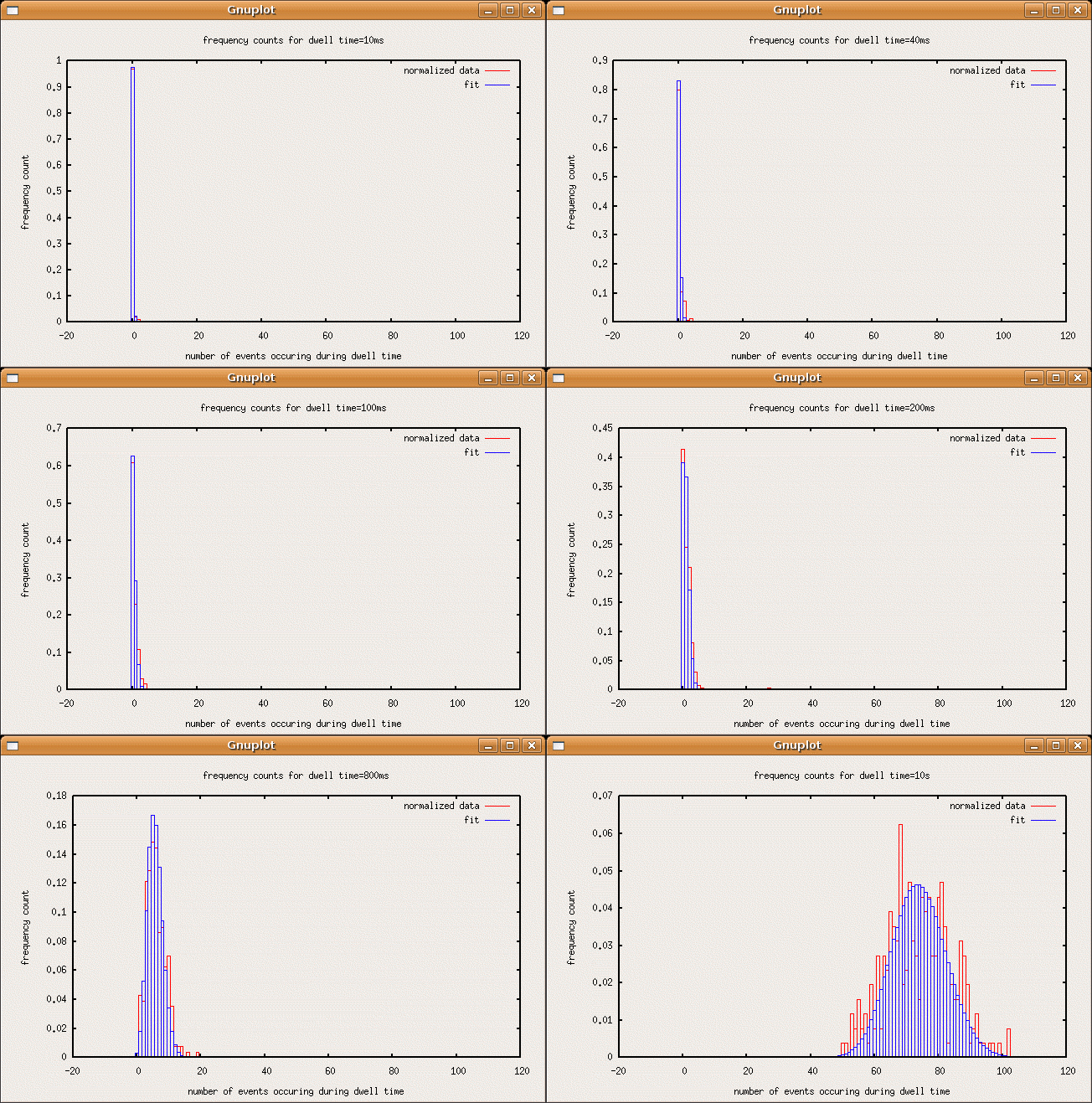
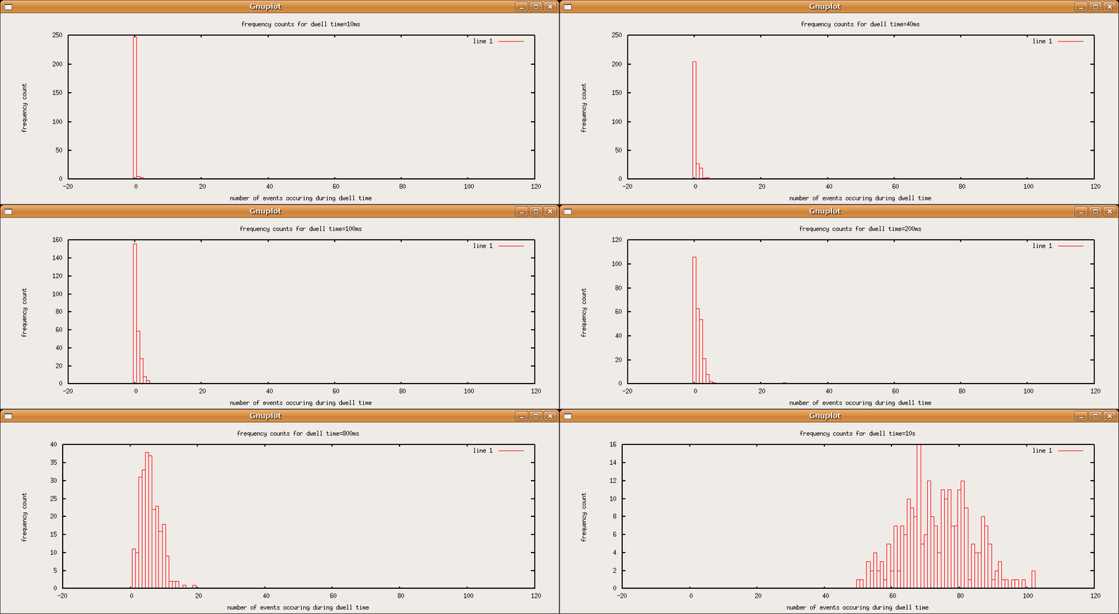
The plot that the script above produced with the data I obtained are shown in sequence below. As the dwell time increases, the most often occurring event count increases and the frequency vs. event count plots drift from something resembling a poisson distibution of a rarely occuring event to a the poisson distribution of a more common event, which resembles a gaussian.SJK 01:40, 22 October 2007 (CDT)

These graphs are very snazzy, and your data certainly are great...however, it's a bit tough to look at the data, because I don't have a way to "play" and "pause" the animated GIF. So, making the individual images available will definitely be necessary in your formal writeup.
I should point out that something interesting happened while we we counting events with a dwell of 200 ms. Our equipment recorded one instance where 27 events happened in that small dwell time. The mode of the data for dwell time=200ms was 0 events, and were were rarely getting counts more than or equal to 5.SJK 01:27, 22 October 2007 (CDT)

Very interesting! Bradley and Nik left the setup going from last Wednesday until today: 100 second bins, going like 5 days or something. I wonder if they will also record a similar occurance (though 27 events may not be obvious in a 100 second bin)?
By the way, you can easily calculate the probability of 27 events happening in a 200 ms window, given your Poisson fit. You can then use this probability to argue about throwing out that data point when fitting. (Also, you should directly state whether you throw the data out or not, and why.)
In Dr. Gold's lab manual, the poisson distribution is a model for the results of experiments that count random events that occur at a definite average rate and the frequency that one should expect to get a certain count number. If the expected average count is [math]\displaystyle{ \lambda }[/math], the probability that one will obtain the result of [math]\displaystyle{ k }[/math] after performing the counting experiment is
[math]\displaystyle{ f(k;\lambda)=\frac{\lambda^k e^{-\lambda}}{k!} }[/math]
So, to fit my data, I will have to normalize my data and find a suitable [math]\displaystyle{ \lambda }[/math] for each data set.
First off, normalize. If the frequency count of an event count [math]\displaystyle{ k }[/math] is [math]\displaystyle{ x_k }[/math], find some normalizing constant [math]\displaystyle{ N }[/math] so that [math]\displaystyle{ \sum_{k=\operatorname{min}\ k}^{\operatorname{max}\ k} \frac{x_k}{N}=1 }[/math]
Then, find [math]\displaystyle{ \lambda }[/math] such that[math]\displaystyle{ \sum_{k=\operatorname{min}\ k}^{\operatorname{max}\ k}\left(f(k,\lambda)-\frac{x_k}{N} \right)^2 }[/math] is a minimum
Duurrrrr... [math]\displaystyle{ N=256 }[/math] because 256 tests were performed each time.
SJK 01:38, 22 October 2007 (CDT)

It appears what you are doing here is a least squares fit of the Poisson distribution to the histogram, which is a great idea. However, I'd have to think some more, but I think maybe you would want a weighting factor in the denominator, perhaps [math]\displaystyle{ \sqrt{x_k} }[/math] (because the uncertainty in #counts is the sqrt(#counts)). Also, though, via talking with Bradley about this lab, I found that in the wikipedia article on Poisson distribution, they show that the maximum likelihood fit is when lambda is set to equal the average counts for the data. In your formal report, you should compare what you did with the much easier maximum likelihood method.
Through an iterative process, I determine [math]\displaystyle{ \lambda }[/math] to be 0.0261205 for dwell=10ms. Ack, I won't go any further, I'll just stop at 6 significant digits for the others too.
- 10ms,0.0261205
- 20ms,0.0736898
- 40ms,0.185892
- 80ms,0.457154
- 100ms,0.468385
- 200ms,0.937453
- 400ms,2.58578
- 800ms,5.74562
- 1s,7.27233
- 10s,73.9022
 SJK 01:44, 22 October 2007 (CDT)

From my glimpses of the moving GIFs, the fits do look good. In addition to being able to look at the individual images, the fits would probably also be easier to see if they were not also bars, but instead were data points, or curves...
how good are these fits, since I decided to stop at 6 sig figs (quite arbitrarily). I suppose I shall quantify this by taking the average of how far off the actual data is from the fit.
I think the formula is [math]\displaystyle{ Error=\frac{\sqrt{\sum_{k=\operatorname{min}\ k}^{\operatorname{max}\ k}\left(f(k,\lambda)-\frac{x_k}{N} \right)^2}}{\sqrt{N}\sqrt{N-1}} }[/math]
- 10ms, 0.0261205, 5.45905*10^-6
- 20ms, 0.0736898, 1.19310*10^-4
- 40ms, 0.185892, 3.28259*10^-4
- 80ms, 0.457154, 5.95464*10^-4
- 100ms, 0.468385, 3.15888*10^-4
- 200ms, 0.937453, 5.23153*10^-4
- 400ms, 2.58578, 5.22450*10^-4
- 800ms, 5.74562, 2.97039*10^-4
- 1s, 7.27233, 2.59775*10^-4
- 10s, 73.9022, 2.96150*10^-4
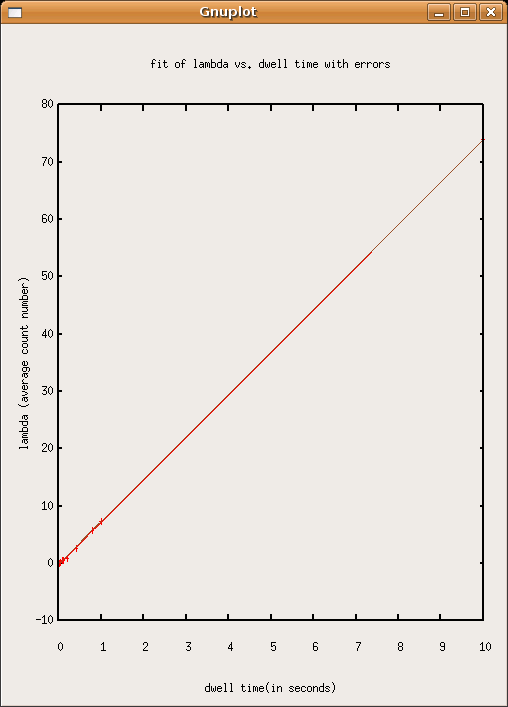
The poisson distribution fits count data of random events that happen at a definite average rate. Therefore [math]\displaystyle{ \frac{\lambda}{dwell time}=some constant }[/math]
A plot of [math]\displaystyle{ \lambda }[/math] vs. dwell time should fit on a line. to do this, I use Dr. Gold's linefit matlab function, modified for use with Octave. (www-hep.phys.unm.edu is down at the moment, maybe provide link when it comes back up or upload modded program here?) SJK 01:38, 22 October 2007 (CDT)

Really cool way to analyze your data (checking lambda versus window width to be linear)!
slope=7.39233+/-0.00003
intercept= -0.048099+/-0.000005
cov(m,b)=0.000000
correlation=0.999983
point error estimate=0.231612
chisq/ndf=265341
So, with our equipment set up the way it was (sorry, no data on this, oops!) we were observing events that occured at an average rate of 7.39 events per second.

