Physics307L F07:People/Knockel/Notebook/071107

Speed of light!

Experimentalists: us

Acknowledgments

Thanks Tomas for help with the software!

Goal

All light travels at the same constant speed, [math]\displaystyle{ c }[/math]=2.998x10⁸ m/s. We want to measure this speed by seeing how the time of travel varies when changing the distance traveled. Measuring this time is difficult since light moves 3/10 of a meter every nanosecond (the distances we can create are only a few meters). Luckily! We have a very sensitive time-to-amplitude converter (TAC) that converts a time interval to a voltage (the voltage is proportional to the time interval). This voltage can easily be measured by a quality oscilloscope.

Equipment

Here is our high-voltage power supply for the PMT (left), our delay box (center), and the TAC (right).

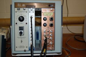
Cool stuff:

• LED that can fire brief pulses of light
• Photomultiplier tube (PMT) to detect the light from the LED
• 2 light polarizers for the PMT and LED
• Delay box (adds a delay on the order of nanoseconds to a signal)
• Time-to-amplitude converter (TAC - pronounced "tack")
• Oscilloscope
• Computer hardware and software that act as a pulse hight analyzer

Boring stuff:

• High-voltage power supply (about 2500 V)
• Low-voltage power supply (about 200 V)
• Many long and short coaxial cables with BNC connectors
• 3 meter tube that LED and PMT can fit inside

Setup

Connecting stuff:

1. Put on the polarizers on the front of the LED and PMT
2. Put the LED and PMT inside opposite sides of the tube facing each other
3. Connect the LED to the low-voltage power supply (power is turned off)
4. Connect the PMT to the high-voltage power supply (power is turned off)
5. Connect the LED and the PMT to the TAC
6. Connect the TAC to the computer
7. Connect the PMT to the oscilloscope

Adjusting stuff:

1. Give the LED about 200 V, but no more than this or it will break
2. Give the PMT 2200 V (no more or it will break) (no less or the TAC will not perceive its signal) (make sure the PMT is in the DARK tube!)
3. Get the oscilloscope to observe the output from the PMT
4. Separate the LED and PMT as much as possible, and then rotate the PMT (thereby rotating the polarizer) so that the PMT signal is the strongest
5. Create 32 ns delay on the delay box (to make sure that the PMT signal always comes AFTER the LED signal)
6. Set the TAC to a range of 100 ns
7. Open the computer software and check to see if the pulses from the TAC are making a Gaussian or Poisson distribution. If not, fiddle with stuff until it does. Make sure the voltage to the PMT is high enough since we had it at only 2000V and we could not get a good signal from the TAC. Keep fiddling and fiddling until you are about to kill Koch for not showing up, and then it will start working. I promise.^{SJK 00:22, 20 November 2007 (CST)}

   

   00:22, 20 November 2007 (CST)
   I did it for your own good, to give you that satisfaction of success and not having to kill Koch

Procedure

We had everything setup as described above, we started by choosing a voltage to keep the PMT's output signal at (the voltage was chosen by rotating the PMT until the polarizers are aligned while the LED and PMT are at a maximum distance). This voltage must be kept constant due to a strange thing called "time walk" that causes weaker signals to have a longer delay. We chose a voltage of -608 units. I think it was measured in volts or maybe millivolts, but I'm not sure, and it doesn't matter because we kept this number constant.

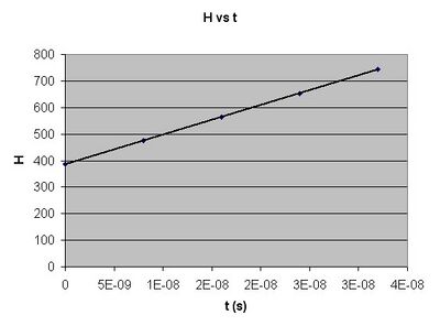
Having chosen a PMT voltage, we needed to calibrate the results from the software. The software measured the average pulse height (H) as well as the full-width-at-half-maximum (FWHM) of the distribution of pulse heights, but it gave these values as dimensionless numbers that were proportional to the voltage of the pulses. Since the TAC made sure the pulses were proportional to the time delay (in fact, given a 100 ns range, 100 ns corresponded to 10 V), the [math]\displaystyle{ H }[/math] is proportional to the time delay (t). To find the proportionality constant (k) where [math]\displaystyle{ H=kt }[/math], we used the delay box to create known delays and then measured the response of [math]\displaystyle{ H }[/math] while keeping everything else the same. The slope of the line plotted from this is [math]\displaystyle{ k }[/math].

Having found [math]\displaystyle{ k }[/math], we knew from the chain rule that

[math]\displaystyle{ c=\frac{dx}{dH}\frac{dH}{dt} }[/math]

and from [math]\displaystyle{ H=kt }[/math] that

[math]\displaystyle{ c=k\frac{dx}{dH} }[/math].

However, since [math]\displaystyle{ x=mH }[/math], where [math]\displaystyle{ m }[/math] is the slope of this line,

[math]\displaystyle{ c=km\, }[/math].

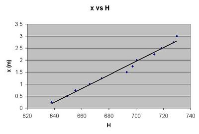
To find [math]\displaystyle{ m }[/math], we simply varied [math]\displaystyle{ x }[/math] and measured the resulting H's. The slope of the line plotted from [math]\displaystyle{ x }[/math] vs. [math]\displaystyle{ H }[/math] gives [math]\displaystyle{ m }[/math]. In doing this, we approximately called the farthest [math]\displaystyle{ x }[/math] as [math]\displaystyle{ x }[/math]=3 meters, and this is not perfect, but we only care about the slope of the plot of [math]\displaystyle{ x }[/math] vs. [math]\displaystyle{ H }[/math], and not the actual values.

For each [math]\displaystyle{ H }[/math] measurement, we made sure the PMT voltage was correct and let the software collect about [math]\displaystyle{ n }[/math]=1,000,000 pulse height measurements.

Lastly, we compared the [math]\displaystyle{ H }[/math] for a certain [math]\displaystyle{ x }[/math] with the PMT at the right to voltage to the [math]\displaystyle{ H }[/math] at the same [math]\displaystyle{ x }[/math] at a very different voltage to get an idea of the amount of error to expect from the "time walk."

Data, Calculations, and Error

For a Gaussian distribution, [math]\displaystyle{ FWHM=2.36\sigma }[/math], where [math]\displaystyle{ \sigma }[/math] is the standard deviation. Using standard error of the mean ([math]\displaystyle{ SE=\frac{\sigma}{\sqrt{n}} }[/math]) to calculate random uncertainty in [math]\displaystyle{ H }[/math], I got a standard error of about 0.035 for every measurement since my [math]\displaystyle{ n }[/math]=1,000,000. Since this value is so small compared to [math]\displaystyle{ H }[/math], I do not provide any random uncertainty error bars in the data below. Also, my random error in the [math]\displaystyle{ x }[/math] measurements is negligible since it is only 1 or 2 millimeters.

I WILL analyze random error in my calculations. This error will simply be the standard error of the slope of the linear regression I do in Excel.

Finding [math]\displaystyle{ k }[/math]

Data

t (ns)	0	8	16	24	32
H	386.6	475.3	563.8	652.8	743.5

[math]\displaystyle{ k=slope=1.114(3)\times10^{10} }[/math] 1/s

Finding [math]\displaystyle{ m }[/math]

Data

x (m)	0.25	0.50	0.75	1.00	1.25	1.50	1.75	2.00	2.25	2.50	2.75	3.00
H	637.9	649.2	655.2	665.8	674.7	693.0	697.3	700.3	713.3	718.6	727.7	729.9

[math]\displaystyle{ m=slope=2.838(11)\times10^{-2} }[/math] m

Finding [math]\displaystyle{ c=km }[/math]

Simply multiplying [math]\displaystyle{ k }[/math] and [math]\displaystyle{ m }[/math] and then propagating the error gives...

[math]\displaystyle{ c=3.16(13)\times10^{8} }[/math] m/s

A closer look at error

The presence of this error is explained by the "time walk," which is the largest source of random error. In our procedure, we altered the PMT voltage from -608 to -856 and noticed that [math]\displaystyle{ H }[/math] decreased by 106, which is larger than the amount it changed throughout the entire 3-meter range. Clearly, the time walk is a huge problem. Since our oscilloscope's averaging ability was not very good and since the oscilloscope would only display discreet voltages (e.g. -600,-608,-614), we could not always make sure the PMT was perfectly at -608, hence the error.

Random error due to not enough significant digits should also make the fit worse and contributed to the error, but this is negligible.

^{SJK 00:28, 20 November 2007 (CST)}

00:28, 20 November 2007 (CST)
Yeah, Excel uses the exact linear regression formulas we talked about in class last month, so you are correct that 32% of the time the accepted value will be outside your range of uncertainty (if your random errors have gaussian distribution).

The actual value of [math]\displaystyle{ c }[/math] is not within my error bars. My uncertainty is 0.13x10⁸ m/s, and the absolute error between the actual and my speed of light is 0.16x10⁸ m/s. This could be due to faulty equipment or some other weird systematic error, but it might not. I am not sure how Excel calculates its standard error of the slope of a linear regression, but perhaps it forms this value so that there is a 68% chance that the correct value is within this distance from the calculated value, so there is a 32% chance that the correct value is not in that interval. Since the actual value of [math]\displaystyle{ c }[/math] is only 1.2 times the standard error, I believe there are no large sources of systematic error.

Conclusion

I have calculated that the speed of light is

[math]\displaystyle{ c=3.16(13)\times10^{8} }[/math] m/s.

The actual value of [math]\displaystyle{ c }[/math]=3.00x10⁸ m/s is slightly outside of the error interval I have provided, but there is no reason why error intervals should include the actual value even if no significant systematic error exists because the actual value is barely outside this interval.^{SJK 00:36, 20 November 2007 (CST)}

00:36, 20 November 2007 (CST)
I like the way your explained it above better: there is a reason to expect it to be in the interval, but 32% of the time it shouldn't. So this is just one of those times, and like you said, it's very close. Great job with this lab! I wonder if your problem initially was that you had the LED too far towards the end? I think you get better data with it closer to the PMT. Good idea with using the time delay generator to calibrate the unknown proportionality. Great presentation of final result...pretty cool that you can get such good data, even with the time walk problem!