Physics307L:People/Ozaksut/Poisson Distribution

Goal

We will use the Poisson, Binomial, and Normal distribution functions to try to analyze data collected by an isolated radiation detector picking up noise (random cosmic events?).

Equipment

Photomultiplier tube

NaI Scintillator

High Voltage Power Supply

Coaxial Cables

Computer

Multichannel analyzer

Theory

I used this lab manual for information [1] When gamma radiation interacts with a NaI crystal, either through the photoelectric effect, Compton scattering, or pair production, photons are created. The photomultiplier tube can then pick up the light signal and transform it into an electric current proportional to the intensity of the incident light. We will use a multichannel analyzer to collect data, and Microsoft Excel to analyze it.

Setup

The PMT is connected to the multichannel analyzer in the computer in multichannel scaling mode, which counts signals, rather than evaluates the intensity of the signals, coming from the PMT. Each channel represents a time bin during which data is collected. We can change the number of channels and the length of time represented by each channel simply using our PCAIII software. After we gather data for a variety of bin time and number of bin combinations, we can upload our data into a program (in my case, Microsoft Excel) to analyze.

Different probability distributions are used to model different situations. The binomial distribution is used to determine the expected successes of an event, given there are only two possible events: (the probability p)= 1- (the other probability q), and the failure of event q is automatically the success of event p.

So, for the following equation, f(k;n,p) is the probability of getting exactly k successes of event K in n tries p is the probability of the success of event K {n\choose k} is all the different ways the k successes out of n tries can be distributed among the n tries (eg. for two successes in three tries, you could have three possible distributions: (success, success, failure), (success, failure, success), or (failure, success, success). 3!/(2!1!) = 6/2 = 3)

[math]\displaystyle{ f(k;n,p)={n\choose k}p^k(1-p)^{n-k} }[/math]

for k = 0, 1, 2, ..., n and where

[math]\displaystyle{ {n\choose k}=\frac{n!}{k!(n-k)!} }[/math]

Wikipedia Binomial distribution

The Gaussian (normal) distribution is modelled by:

[math]\displaystyle{ G(x)=\frac{1}{\sqrt{2\pi\sigma^2}}e^{-\frac{\left(x-a\right)^2}{2\sigma^2}} }[/math]

[math]\displaystyle{ a }[/math] = mean, [math]\displaystyle{ \sigma }[/math] = standard deviation.

\sigma is the standard deviation, or variance in probability, of the distribution, defined to be

[math]\displaystyle{ \sigma = \sqrt{\int (x-\mu)^2 \, p(x) \, dx} }[/math]

and \mu is the expected value

The Poisson distribution,

[math]\displaystyle{ P(x)=e^{-a}\frac{a^x}{x!} }[/math]

with a standard deviation of

[math]\displaystyle{ \sigma=\sqrt{a} }[/math],

where a is the expected number of events per time interval, has a unique feature: it's standard deviation is the square root of the mean value ([math]\displaystyle{ \sqrt{a} }[/math]). If p or q in the binomial distribution is very small, or if the number of trials is very large, it resembles the poisson distribution.

If the average number of events per time interval is large, the poisson distribution and normal distribution resemble each other.

For modelling cosmic events, which occur randomly but have a definite average rate of occurence, the best distribution function to use to model the events would depend on the average number of events per time interval and the number of trials performed.

Results

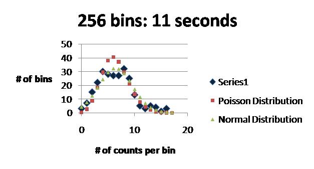
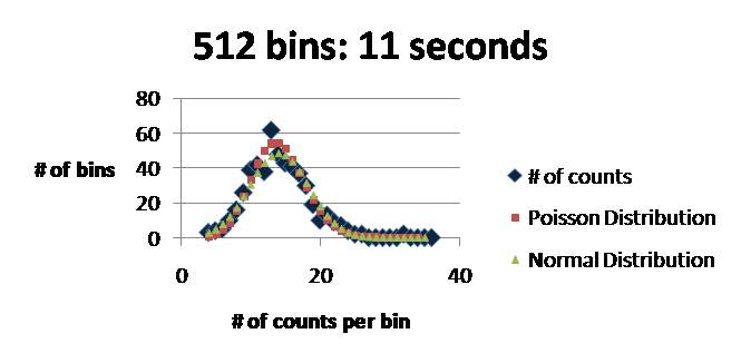
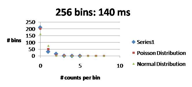
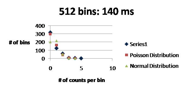
Please see this file for spreadsheets of all data collected: Media:anniemattpoisson.xlsx The following data sets have been contrasted with normal distribution and poisson distribution curves.

Conclusion

Clearly, for random events occurring at definite average frequencies, Poisson distribution curves best model real behavior for short time intervals. For larger time intervals, such as the 11 second data sets, it is unclear whether Poisson or normal distribution curves better fit the actual data, but this lab illustrates that as the number of bins increases, poisson and normal distribution curves better resemble each other.

Improvements?

Next time, I'd take more data at intermediate bin times. Also, I'd be really careful about labelling my files at the lab station, because the bin time and number of bins isn't included in the file.

Between you and me, I'm not totally sure I understand how random events can be modelled with the binomial distribution function... We don't want small probability or many trials, otherwise we might as well use the poisson, but i'm not sure how to get p~q. For small bin times, you'll get a lot of 0's and a few not-0's. For large bin times, like the 11 seconds, you get a smooth distribution around some number, but if you calculate the probability of getting any of those numbers, you'll still have way more "other numbers" than the number you're calculating the probability of getting... I understand the binomial distribution for explicit yes-no options, but for this experiment...not so much.

Steve Koch 00:44, 4 December 2007 (CST):Yeah, it appears that it is most common to derive the Poisson distribution by starting with the Binomial and then making approximation (take the number of trials to infinity, and the probability of success to zero, while holding the number of success fixed). You can also derive it by assuming a constant chance of something happening per unit time, and then integrating. OK, but in terms of the binomial approximation, a good way of understanding it (for me) is to think about a chunk of radioactive material from which you are detecting about 1 decay per second. In this chunk, you might have 10^23 or more atoms, so in one second, the chance of any of them decaying is tiny, but the number of "trials" is huge. You can think of each time bin as a binomial experiment: you're flipping 10^23 coins, and expect 99.9999...9999999% to be heads (don't decay) and 0.000000...00001% to be tails (decay). The statistics of this would be determined by the binomial distribution, but the Poisson is an excellent approximation (as you can find on wikipedia and elsewhere). In your case, you are probably looking at uncorrelated cosmic events, in which case it's harder to think about what the binomial experiment would mean. However, the cosmic events have the same behavior as the radioactive decays, meaning they are completely uncorrelated (hopefully...as long as there is no time dependence).