Physics307L:People/Gooden/Formal Lab Report
- MEASUREING THE SPEED OF LIGHT ELECTRONICALLY
SJK 16:14, 12 November 2007 (CST)

You will want a more formal title. Something more descriptive, "Measuring the speed of light by blah blah blah.
Matthew E. Gooden, Zane Gibson
UNM Department of Physics
Abstract
SJK 16:17, 12 November 2007 (CST)
Good start on the abstract, but needs to be expanded. Take a look at Today's lecture for discussion of what should be in the abstract. In addition to what you have, need to add motivation, how you did it, and conclusions (future work)
- The objective of this experiment was to determine the value of c, the speed of light. We have measured [math]\displaystyle{ c=\left(2.83 \pm .23\right)\times10^8 m/s }[/math] in good agreement with the accepted value of [math]\displaystyle{ 2.99\times10^8 {m/s} }[/math].
Introduction
SJK 16:23, 12 November 2007 (CST)
This is a great start on the introduction, in particularly explaining the motivation for why speed of light is important. You will want to add citations to original research reports (for example, Einstein's 1905 paper, since you talk about it), and also a citation to any other background material you used (e.g. wikipedia). But the citations to original research articles is most important.
Also, you need to add background on how people have measured the speed of light (the different methods), and then finally mention how you measured the speed of light.
Also, you need to use a more formal tone. For example "...but FINITE!" is too informal.
- We investigated the Speed of Light during this experiment. The speed of light is just what it sounds,How fast light Travels! The speed of light historically have been very fascinating. It was once believed that light travels instantaneously between locations, that its speed was infinite. However, once physicists began investigating more and they discovered that light's speed is very very large, but FINITE! and specifically it is around 300 million meters per second by todays calculations. Physicists also believed that light followed Galilean relativity/motion and that its speed was always dependent upon how fast you were traveling. However, Albert Einstein showed in 1905 with Special Relativity that the speed of light is a constant, that it never changes for anyone/anything no matter how fast you move. The speed of light c, can also be found in dealing with the energy of photons, special relativity and the lorentz transformations and many other areas of physics. As one can tell this constant plays a very big role in physics.
Methods and Materials
SJK 16:27, 12 November 2007 (CST)
The phrase you use is sort of informal. Try instead making a sub-heading, "Required Equipment" and then listing the equipment (plus model numbers and manufacturers). Also, typically things aren't written with numbered steps, but are more likely to break things up into sub-headings. Take a look at some published papers in Physical Review B to get an idea of how they are written.
Also, missing from the methods is a description of your data analysis methods. It is very important to state what methods you used and any associated software (Matlab).
- This experiment requires the use of a lot of different equipment:
Time-Amplitude Converter (TAC)
LED
Photomultiplier Tube (PMT)
DC Power supply (150V-200V) - LED
DC Power supply (1800V-2000V) - PMT
Oscilloscope
Delay box
Several Meter Sticks
Long Tube
Procedure {{SJK comment|l=16:59, 12 November 2007 (CST)|c=This is actually a nice detailed "how to," but unfortunately isn't quite the correct style for a formal report. Even though the purpose is to allow people to reproduce your experiments, you don't write it in a "here's how you do it," but rather, "this is what we did". To make this easier, you should draw a schematic with all the connections, and then you can say, "we connected the instruments as in "figure ____".
- 1) WARNING:Never expose the PMT to direct light while power source is on, this will destroy the PMT.
- 2) To begin you must connect the power supplies to both the LED and the PMT that are at either ends of the tube; the low and high voltage supplies respectively.
- 3) With the PMT in the left end of the tube near the equipment, attatch the meter sticks to the LED and insert it into the right end of the tube.You will want to tape or fasten the meter sticks together to be able to move the LED a sufficient distance.
- 4) Then connect the LED to the TAC's start jack with a BNC cable, and also connect the PMT to the stop jack on the TAC with another BNC cable. Next you also want to run a cable from the PMT to the oscilloscope's Channel 1 and from the TAC to channel 2 on the oscilloscope.
- The oscilloscope will measure the voltage output from the PMT on channel 1 and the signal from the TAC will respresent the time delay that you want to be measuring.
- 5) You now want to adjust the oscilloscope to be able to see the signals from the PMT and LED. On channel 1 of the Oscilloscope you are wanting to see a level curve with a sudden drop in potential and then a rise back up. On channel 2 the signal from the TAC should look like a semi-square wave that is oscillating up and down rather rapidly.
- 6) Once all set up, you want to pick a value of the voltage on Ch 1 and attempt to maintain that value for your measurments. This is accomplished by turning the PMT left/right to allign or unallign its polarizer with that of the LED.
- 7) Next, using the aquire button on the oscilloscope you can choose to average over the values that the oscilloscope is recieving to allow you to take measurments. You want to choose the 128 setting under the average command, so the signal is more stable. Then use the measure function to allow you to see the values outputed to channels 1 and 2 to make your measurments. Looking for the minimum on channel 1 and maximum on channel 2.
- 8) Now we can start making measurments! - to do this you must pick your desired value for channel 1 and then holding the PMT steady have your partner pull or push the meter stick connected to the LED in or out of the tube. Record how far the meter stick moved relative to the opening of the tube and then readjust the PMT so that channel 1 on the oscilloscope returns to your previously picked value.Then simply continue.
- For this experiment, we are not concerned with the actual distance between the PMT and LED. Which can seem a little strange. Rather at any particular distance between the PMT and LED we make a measurment and then we are only concerned with the change in that distance for the next measurment, since we are measuring the time delay of the signal from the LED pulse and the PMT signal.
SJK 17:00, 12 November 2007 (CST)
Great pictures and good start on the captions. Probably more detail in the captions to make sure people know which piece of equipment they are supposed to look at.
-
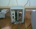 From left: power supply for photomultiplier, delay box, TAC (time amplitude converter)
 -
 Power supply for LED light emitter.
 -
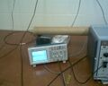 oscilloscope
 -
 On top tried different time delay to try and get better signal.


Results and Discussion
SJK 17:04, 12 November 2007 (CST)
The tables and figures are great, but they need captions and labels. The captions should allow a reader to look at a figure (or table) and understand what it is without reading the main text. In the main text, you need more detail. Instead of saying "in the table below, we give our data," you should say, "Table 1 shows the results of experiment 1, in which the PMT was kept at ___ for distances between ___ and ___. The linear fit to these data (as explained in methods) is shown in Figure ___. Basically, it looks like you have three different sets of data, so you should explain what the three sets are, and then either in this section or the next section, explain which data set is the best, etc.
- In the tables below we give our data, that was obtained from the experiment. Immediately afterwards we will detail our analysis and present our final results that were mentioned above.
- In analyzing the data we used the equation :[math]\displaystyle{ V = G*T }[/math] to relate the voltages to time, with G=1/10 volts/nanosecond
| Data Set 1 Measurments | PMT Ch1 Voltage | TAC Time delay voltage | Distance (cm) | Time (ns) |
|---|---|---|---|---|
| 1 | [math]\displaystyle{ 600 \pm 8 {mV} }[/math] | [math]\displaystyle{ 3.24\pm.04 }[/math] | 60 | 32.4 |
| 2 | [math]\displaystyle{ 600 \pm 8 {mV} }[/math] | [math]\displaystyle{ 3.2 \pm.04 }[/math] | 80 | 32 |
| 3 | [math]\displaystyle{ 600 \pm 8 {mV} }[/math] | [math]\displaystyle{ 3.08 \pm.04 }[/math] | 100 | 30.8 |
| 4 | [math]\displaystyle{ 600 \pm 8 {mV} }[/math] | [math]\displaystyle{ 3.00 \pm.04 }[/math] | 120 | 30 |
| 5 | [math]\displaystyle{ 600 \pm 8 {mV} }[/math] | [math]\displaystyle{ 2.96\pm.04 }[/math] | 140 | 29.6 |
| 6 | [math]\displaystyle{ 600 \pm 8 {mV} }[/math] | [math]\displaystyle{ 3.00 \pm.04 }[/math] | 130 | 30 |
| 7 | [math]\displaystyle{ 600 \pm 8 {mV} }[/math] | [math]\displaystyle{ 3.12 \pm.04 }[/math] | 90 | 31.2 |
| 8 | [math]\displaystyle{ 600 \pm 8 {mV} }[/math] | [math]\displaystyle{ 3.2 \pm.04 }[/math] | 70 | 32 |
| Data Set 2 Measurments | PMT Ch1 Voltage | TAC Time delay voltage | Distance (cm) | Time (ns) |
|---|---|---|---|---|
| 1 | [math]\displaystyle{ 800 \pm 8 {mV} }[/math] | [math]\displaystyle{ 2.44\pm.04 }[/math] | 70 | 24.4 |
| 2 | [math]\displaystyle{ 800 \pm 8 {mV} }[/math] | [math]\displaystyle{ 2.4 \pm.04 }[/math] | 80 | 24 |
| 3 | [math]\displaystyle{ 800 \pm 8 {mV} }[/math] | [math]\displaystyle{ 2.36 \pm.04 }[/math] | 90 | 23.6 |
| 4 | [math]\displaystyle{ 800 \pm 8 {mV} }[/math] | [math]\displaystyle{ 2.32 \pm.04 }[/math] | 100 | 23.2 |
| 5 | [math]\displaystyle{ 800 \pm 8 {mV} }[/math] | [math]\displaystyle{ 2.32\pm.04 }[/math] | 110 | 23.2 |
| Data Set 3 Measurments | PMT Ch1 Voltage | TAC Time delay voltage | Distance (cm) | Time (ns) |
|---|---|---|---|---|
| 1 | [math]\displaystyle{ 720 \pm 8 {mV} }[/math] | [math]\displaystyle{ 2.8\pm.04 }[/math] | 27.5 | 28 |
| 2 | [math]\displaystyle{ 720 \pm 8 {mV} }[/math] | [math]\displaystyle{ 2.64 \pm.04 }[/math] | 70 | 26.4 |
| 3 | [math]\displaystyle{ 720 \pm 8 {mV} }[/math] | [math]\displaystyle{ 2.52 \pm.04 }[/math] | 110 | 25.2 |
| 4 | [math]\displaystyle{ 720 \pm 8 {mV} }[/math] | [math]\displaystyle{ 2.44 \pm.04 }[/math] | 130 | 24.4 |
| 5 | [math]\displaystyle{ 720 \pm 8 {mV} }[/math] | [math]\displaystyle{ 2.72\pm.04 }[/math] | 50 | 27.2 |
- Once we collected the data above from the three different trials we began our data analysis using Microsoft Excell and Matlab to perform least-squares fits to the data, find our error and produce plots of the data.
- Here are the plots of our data given above,where the slope of the least-squares line respresents the speed of light approximation by the data:

- After performing the least-squares analysis on each data set we were able to come up with these values for the speed of light C for each set along with the suspected error.
- Data Set 1
[math]\displaystyle{ c=\left(2.68 \pm 0.18\right)\times10^{8} m/s }[/math]
- Data Set 2
[math]\displaystyle{ c=\left(2.94 \pm 0.42\right)\times10^{8} m/s }[/math]
- Data Set 3
[math]\displaystyle{ c=\left(2.89 \pm 0.08\right)\times10^{8} m/s }[/math]
SJK 17:16, 12 November 2007 (CST)
Two things I want you to do: (1) learn how to perform a weighted average when combining these three values. This weights the value obtained with better precision more highly. (2) Decide whether you believe one data set more than the others, and then make a plan for taking the best data possible, and then take that data set.
- By averaging the three values above for the speed of light and taking this to be our final value for this experiment,we find that the speed of light is:
- [math]\displaystyle{ c=\left(2.83 \pm .23\right)\times10^8 m/s }[/math]
Conclusions
SJK 17:07, 12 November 2007 (CST)
This first sentence is too informal. Readers will assume you are pleased with your result, if you are publishing it, so instead you should comment on how it compares with the accepted value, and you don't have to say "unlike most experiments."
- With our value of the Speed of Light c, we are fairly happy with the result. Unlike most experiments however we do know the true value for c, and so we can look at the relative error between the accepted value and our reported value, which is given by:
[math]\displaystyle{ Relative Error=\frac{\left|2.99\times10^{8}-c\right|}{\left|2.99\times10^{8}\right|}=0.0535=5.3% }[/math]
- With this result we are very pleased with the outcome of the experiment.
- Given the 5% error in the measurment, we can see that there is error in our measurments and the experiment. If we had more time we would have liked to make several more sets of measurments to use in our analysis, and also to improve on how the distance measurments were done and the apparatus was set up. The LED fit into the tube very tighly and this caused the tube to be shifted and/or rotated when the LED was pulled or pushed out the tube to change the distance between it and the PMT. Also, the area that the experiment was set up on was not suitable or desirable to perform the experiment. The PMT end of the tube was set on an extra piece of equipment balanced on its power cord and set up in such a way that reaching out and holding the PMT still and also rotating it to align its polarizer with the LED was difficult. If we were to redo the experiment in the future we would attempt to fix the problems in how the experiment was set up,which would hopefully allow more accurate measurments to be taken and reduce the error.
Acknowledgments
SJK 17:13, 12 November 2007 (CST)
Aww, thanks :p. OK, so for this part you also want to keep it formal (phrase "why we don't care..."). In a real paper it's very important to acknowledge those who helped but who aren't authors. It does seem a little silly to acknowledge your lab instructor, but I guess you should keep it in. You could shorten it, though, and leave out the specifics. ("We thank Dr. Koch (and whoever else) for their help with the instrumentation and data anslysis.") In a real paper, often specifics are left out, but sometimes it is good to be specific.
- We would like to acknowledge Dr. Koch for his help in explaining how equipment such as the TAC and PMT operated so that we could have a better understanding of what was happening. He also was able to explain the signals from the LED and PMT and why we dont care about the actual distance between the PMT and LED but only the change in that distance at each measurment. Dr. Koch was a very valuable asset in performing this experiment.
References
- Dr. Golds Physics 307L lab manual, which can be found here:
- EG&G Ortec TAC Operator Manual, which can be found in the Senior Lab
- Antonio Rivera's Lab Notebook:
Koch comments
Overall, I think your data and analysis are good, which is a great thing, because that is the heart of a good report, of course. However, the report needs significant work in a lot of areas, as noted above throughout. Some sections had good starts, but needed more info (such as introduction) and in many other places, the style is not what it should be for a formal report. You should make significant revisions and then get more feedback from me before submitting the final version. Additionally, in order to get an outstanding grade, I will want you to take more measurements, trying to obtain even better data than you have already. Some notable things:
- Need many more citations (as discussed in class)
- Take a look at several published articles to get a feel for the formal writing. You need to emulate this (e.g., not written as bulleted lists, etc.)
