Physics307L:People/Gibson/Formal Lab Report
SJK 13:27, 18 November 2007 (CST)

You are missing a title, author & contact info! Overall, you have really great data and nice presentation of the data and results. But as far as a formal report goes, many things are missing or need to be made more formal. A good thing to do will be to look at published papers, (here for example, make sure it's an experimental report, not theory) to get an idea of how it's done. Also, as I mention below, to get an outstanding grade, I'll want you to try to get even better data, as you mention.
Abstract
SJK 13:27, 18 November 2007 (CST)
This is more like a methods section than an abstract. See this page for a brief explanation of abstract. It should be a brief summary of the entire paper: motivation, brief methods statement, result (your best fit value), conclusion.
In our examination of determining the speed of light, we used several key components to help us measure this interesting constant. We first used a dark 3 meter or so long tube in which an LED (light emitting diode) and a PMT (photo multiplier tube) were placed on opposite ends. The necessity for darkness in the room was not needed seeing as the tube was exactly the diameter of both pieces of equipment used blocking all outside light from potentially adding error to the experiment. What the PMT does is measure a voltage it receives from the LED and reports it to an outside source like an oscilloscope. From here we can create various wave propagations and plot them; in addition to this the oscilloscope is also used to measure the signal coming from the TAC (Time Amplitude Converter) which is receiving a signal from the LED. These two plots (voltage and signal) are averaged as best as they can be to find a steady voltage for each piece respectively to begin taking data.
Introduction
SJK 13:37, 18 November 2007 (CST)
This introduction is far too short. See other students for examples of introductions (such as Jesse's report). See this page for explanation. When you fix your introduction, you will need to include many references to original research publications.
In this experiment we examined how closely we could reach the theoretical value of the speed of light. This result is actually very interesting to researchers that use the speed of light in experiments of their own.
The speed of light was first seen as a constant by Einstein in 1905 with his introduction of the Theory of Special Relativity.
Methods and Materials
SJK 13:43, 18 November 2007 (CST)
This is a great start on materials and methods...the main problem is just that it's not the right style for materials and methods of a formal report. Check out some publications and you will start to get an idea for how they are written. One main comment is that you write a procedure as a "how to" whereas usually in a formal publication, you write it as a "we did this". For example, instead of saying, "to begin, you must connect power supplies..." you would say, "We first connected the high voltage power supply (company and model number) to the PMT (voltage setting ___). Next we connected the LED power supply (company and model number). In this way, you work in the equipment list into the methods. Also, as I pointed out, make sure you include all brands and model numbers. Also, you also need to discuss your data analysis methods and what software you use to do the fits.
The equipment used is explained in this list:
- Time-Amplitude Converter (TAC)
- Light Emitting Diode (LED)
- Photomultiplier Tube (PMT)
- DC Power supply (150V-200V) - LED
- DC Power supply (1800V-2000V) - PMT
- Oscilloscope
- Time Delay Apparatus
- 3 Meter sticks
- 3 Meter Long Tube
Procedure for setting up
- 1) WARNING:Never expose the PMT to direct light while power source is on, this will destroy the PMT.
- 2) To begin you must connect the power supplies to both the LED and the PMT that are at either ends of the tube; the low and high voltage supplies respectively.
- 3) With the PMT in the left end of the tube near the equipment, attach the meter sticks to the LED and insert it into the right end of the tube. You will want to tape or fasten the meter sticks together to be able to move the LED a sufficient distance.
- 4) Then connect the LED to the TAC's start jack with a BNC cable, and also connect the PMT to the stop jack on the TAC with another BNC cable. Next you also want to run a cable from the PMT to the oscilloscope's Channel 1 and from the TAC to channel 2 on the oscilloscope.
- The oscilloscope will measure the voltage output from the PMT on channel 1 and the signal from the TAC will represent the time delay that you want to be measuring.
- 5) You now want to adjust the oscilloscope to be able to see the signals from the PMT and LED. On channel 1 of the Oscilloscope you are wanting to see a level curve with a sudden drop in potential and then a rise back up. On channel 2 the signal from the TAC should look like a semi-square wave that is oscillating up and down rather rapidly.
- 6) Once all set up, you want to pick a value of the voltage on Ch 1 and attempt to maintain that value for your measurements. This is accomplished by turning the PMT left/right to align or unalign its polarizer with that of the LED.
- 7) Next, using the acquire button on the oscilloscope you can choose to average over the values that the oscilloscope is receiving to allow you to take measurements. You want to choose the 128 setting under the average command, so the signal is more stable. Then use the measure function to allow you to see the values outputted to channels 1 and 2 to make your measurements. Looking for the minimum on channel 1 and maximum on channel 2.
- 8) Now we can start making measurements! - to do this you must pick your desired value for channel 1 and then holding the PMT steady have your partner pull or push the meter stick connected to the LED in or out of the tube. Record how far the meter stick moved relative to the opening of the tube and then readjust the PMT so that channel 1 on the oscilloscope returns to your previously picked value.Then simply continue.
- For this experiment, we are not concerned with the actual distance between the PMT and LED. Which can seem a little strange. Rather at any particular distance between the PMT and LED we make a measurement and then we are only concerned with the change in that distance for the next measurement, since we are measuring the time delay of the signal from the LED pulse and the PMT signal.
SJK 14:43, 18 November 2007 (CST)
Good figures; captions should be more descriptive and more formal. For example, "Digital oscillscope used for monitoring the voltage level from the anonde of the PMT..."
Also, you should have a schematic of the setup.
-
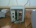 From left: power supply for photomultiplier, delay box, TAC (time amplitude converter)
 -
 Power supply for LED light emitter.
 -
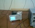 oscilloscope
 -
 On top tried different time delay to try and get better signal.


Results and Discussion
SJK 13:49, 18 November 2007 (CST)
Your data are excellent! This section, though, is too informal. Again, take a look at some published papers to get a feel for what is typical. Some discussion you can include is what are the sources of your uncertainties, what (if any) are the differences in the data sets..
In discovering the times for each data set, we were required (since we didn't measure time) to use the equation V=G*T where V is voltage; T is the time we want, and G is a constant set before we began taking measurements = 1/10 volt/nanosecond.
Here we took down measurements as listed in the procedure and placed them below:
SJK 13:45, 18 November 2007 (CST)
These are great tables! You need to label them "Table 1" etc. and then in the text of your Results and Discussion section, you refer to them as "...as shown in Table 1"
| Data Set 1 Measurments | PMT Ch1 Voltage | TAC Time delay voltage | Distance (cm) | Time (ns) |
|---|---|---|---|---|
| 1 | [math]\displaystyle{ 600 \pm 8 {mV} }[/math] | [math]\displaystyle{ 3.24\pm.04 }[/math] | 60 | 32.4 |
| 2 | [math]\displaystyle{ 600 \pm 8 {mV} }[/math] | [math]\displaystyle{ 3.2 \pm.04 }[/math] | 80 | 32 |
| 3 | [math]\displaystyle{ 600 \pm 8 {mV} }[/math] | [math]\displaystyle{ 3.08 \pm.04 }[/math] | 100 | 30.8 |
| 4 | [math]\displaystyle{ 600 \pm 8 {mV} }[/math] | [math]\displaystyle{ 3.00 \pm.04 }[/math] | 120 | 30 |
| 5 | [math]\displaystyle{ 600 \pm 8 {mV} }[/math] | [math]\displaystyle{ 2.96\pm.04 }[/math] | 140 | 29.6 |
| 6 | [math]\displaystyle{ 600 \pm 8 {mV} }[/math] | [math]\displaystyle{ 3.00 \pm.04 }[/math] | 130 | 30 |
| 7 | [math]\displaystyle{ 600 \pm 8 {mV} }[/math] | [math]\displaystyle{ 3.12 \pm.04 }[/math] | 90 | 31.2 |
| 8 | [math]\displaystyle{ 600 \pm 8 {mV} }[/math] | [math]\displaystyle{ 3.2 \pm.04 }[/math] | 70 | 32 |
| Data Set 2 Measurments | PMT Ch1 Voltage | TAC Time delay voltage | Distance (cm) | Time (ns) |
|---|---|---|---|---|
| 1 | [math]\displaystyle{ 800 \pm 8 {mV} }[/math] | [math]\displaystyle{ 2.44\pm.04 }[/math] | 70 | 24.4 |
| 2 | [math]\displaystyle{ 800 \pm 8 {mV} }[/math] | [math]\displaystyle{ 2.4 \pm.04 }[/math] | 80 | 24 |
| 3 | [math]\displaystyle{ 800 \pm 8 {mV} }[/math] | [math]\displaystyle{ 2.36 \pm.04 }[/math] | 90 | 23.6 |
| 4 | [math]\displaystyle{ 800 \pm 8 {mV} }[/math] | [math]\displaystyle{ 2.32 \pm.04 }[/math] | 100 | 23.2 |
| 5 | [math]\displaystyle{ 800 \pm 8 {mV} }[/math] | [math]\displaystyle{ 2.32\pm.04 }[/math] | 110 | 23.2 |
| Data Set 3 Measurments | PMT Ch1 Voltage | TAC Time delay voltage | Distance (cm) | Time (ns) |
|---|---|---|---|---|
| 1 | [math]\displaystyle{ 720 \pm 8 {mV} }[/math] | [math]\displaystyle{ 2.8\pm.04 }[/math] | 27.5 | 28 |
| 2 | [math]\displaystyle{ 720 \pm 8 {mV} }[/math] | [math]\displaystyle{ 2.64 \pm.04 }[/math] | 70 | 26.4 |
| 3 | [math]\displaystyle{ 720 \pm 8 {mV} }[/math] | [math]\displaystyle{ 2.52 \pm.04 }[/math] | 110 | 25.2 |
| 4 | [math]\displaystyle{ 720 \pm 8 {mV} }[/math] | [math]\displaystyle{ 2.44 \pm.04 }[/math] | 130 | 24.4 |
| 5 | [math]\displaystyle{ 720 \pm 8 {mV} }[/math] | [math]\displaystyle{ 2.72\pm.04 }[/math] | 50 | 27.2 |
- NOTE: See acknowledgments section
Once we completed calculating our times for each of the trials, we then proceeded to construct 3 least squares plots to determine what our value of the speed of light would be. To do this we simply took the distance recorded vs time which then gave us a very linear graph... the slope of this line is the constant we were looking for.

SJK 13:46, 18 November 2007 (CST)
Great job with reporting your final values, nice use of significant figures, easy to read!
- The slopes for each data set are listed below:
Data Set 1
[math]\displaystyle{ c=\left(2.68 \pm 0.18\right)\times10^{8} m/s }[/math]
Data Set 2
[math]\displaystyle{ c=\left(2.94 \pm 0.42\right)\times10^{8} m/s }[/math]
Data Set 3
[math]\displaystyle{ c=\left(2.89 \pm 0.08\right)\times10^{8} m/s }[/math]
SJK 13:29, 18 November 2007 (CST)
For the final version, I want you to learn how to do a weighted average of these values (where you weight each data set by the uncertainty in that data set).
Average of all three data sets:
[math]\displaystyle{ c=\left(2.83 \pm .23\right)\times10^8 m/s }[/math]
From here we calculated our relative error to determine the amount off of the theoretical value:
[math]\displaystyle{ Relative Error=\frac{\left|2.83\times10^{8}-2.99\times^{8}\right|}{\left|2.99\times10^{8}\right|}=0.0535=5.3% }[/math]
Conclusions
Our average value for the speed of light was extremely close to the theoretical value! Given the ambiguity of how the measurements where taken the result was quite surprising to say the least. A relative error of 5.3% is more than acceptable for this situation.
Given that we were only off by ~5% this leads us to believe that if we has had more time to conduct additional measurements we would be able to shrink this as much as 1% or so.SJK 13:30, 18 November 2007 (CST)
Great! I want you to make a plan for how to take the best data possible, and then carry out the experiment before you turn in your final version!
Acknowledgments
SJK 13:33, 18 November 2007 (CST)
Thank you for the acknowledgments here. You can be less specific, though, in a formal report. Something like "We thank Steve Koch for help with instrumentation and experiment design.
As for thanking Matt, in a real research paper, you would probably be co-authors with Matt, so it is customary not to list him in the acknowledgments. In this case, since he is not a co-author, you can say "we thank Matt Gooden for help with data acquisition, data analysis, and data presentation." But put those in your own words.
We would first like to thank Dr. Koch for his help in the beginning to understand how each pieces of equipment worked such as the time-delay and the TAC. He also helped us (Matt Gooden and I) understand physically as well as mathematically why how far the LED is away from the end of the tube doesn't matter as much as the change in distance. Dr. Koch was a key element in completing this experiment and understanding it.
On an additional note, I would like to thank Matt, my lab partner for his perseverance in figuring out the tables listed in the Results and Discussions section. These were quite a pain with the wiki editing interface and the reader would benefit more from the tables then standard reporting of the values.
References
SJK 13:34, 18 November 2007 (CST)
You will need to have a lot more references, of course. These will need to be to original research publications. Most references will be cited in your introduction and methods.
Dr. Golds Physics 307L lab manual for setting up the experiment, which can be found here: Previous Course lab manual.
