Lab Notebook Kevin McGee
5/18/2015
Microarray Data analysis Workflow
- Set browser to send downloads to Desktop
- Followed the Protocal found on OpenWetWare:
Installing R 3.1.0 and the limma package
The following protocol was developed to normalize GCAT and Ontario DNA microarray chip data from the Dahlquist lab using the R Statistical Software and the limma package (part of the Bioconductor Project).
- The normalization procedure has been verified to work with version 3.1.0 of R released in April 2014 (link to download site) and and version 3.20.1 of the limma package ( direct link to download zipped file) on the Windows 7 platform.
- Note that using other versions of R or the limma package might give different results.
- Note also that using the 32-bit versus the 64-bit versions of R 3.1.0 will give different results for the normalization out in the 10-13 or 10-14 decimal place. The Dahlquist Lab is standardizing on using the 64-bit version of R.
- To install R for the first time, download and run the installer from the link above, accepting the default installation.
- To use the limma package, unzip the file and place the contents into a folder called "limma" in the library directory of the R program. If you accept the default location, that will be C:\Program Files\R\R-3.1.0\library (this will be different on the computers in S120 since you do not have administrator rights).
Running the Normalization Scripts
- Create a folder on your Desktop to store your files for the microarray analysis procedure.
- Download the zipped file that contains the
.gprfiles and save it to this folder (or move it if it saved in a different folder).- Unzip this file using 7-zip. Right-click on the file and select the menu item, "7-zip > Extract Here".
- Download the GCAT_Targets.csv file and Ontario_Targets_wt-dCIN5-dGLN3-dHAP4-dHMO1-dSWI4-dZAP1-Spar_20150514.csv files and save them to this folder (or move them if they saved to a different folder).
- Download the Ontario_Chip_Within-Array_Normalization_modified_20150514.R script and save (or move) it to this folder.
- Download the Within-Array_Normalization_GCAT_and_Merged_Ontario-GCAT_Between-Chip_Normalization_modified_20150514.R script and save (or move) it to this folder.
Within Array Normalization for the Ontario Chips
- Launch R x64 3.1.0 (make sure you are using the 64-bit version).
- Change the directory to the folder containing the targets file and the GPR files for the Ontario chips by selecting the menu item File > Change dir... and clicking on the appropriate directory. You will need to click on the + sign to drill down to the right directory. Once you have selected it, click OK.
- In R, select the menu item File > Source R code..., and select the Ontario_Chip_Within-Array_Normalization_modified_20150514.R script.
- You will be prompted by an Open dialog for the Ontario targets file. Select the file Ontario_Targets_wt-dCIN5-dGLN3-dHAP4-dHMO1-dSWI4-dZAP1-Spar_20150514.csv and click Open.
- Wait while R processes your files.
Within Array Normalization for the GCAT Chips and Between Array Normalization for All Chips
- These instructions assume that you have just completed the Within Array Normalization for the Ontario Chips in the section above.
- In R, select the menu item File > Source R code..., and select the Within-Array_Normalization_GCAT_and_Merged_Ontario-GCAT_Between-Chip_Normalization_modified_20150514.R script.
- You will be prompted by an Open dialog for the GCAT targets file. Select the file GCAT_Targets.csv and click Open.
- Wait while R processes your files.
- When the processing has finished, you will find two files called GCAT_and_Ontario_Within_Array_Normalization.csv and GCAT_and_Ontario_Final_Normalized_Data.csv in the same folder.
- Save these files to LionShare and/or to a flash drive.
Visualizing the Normalized Data
Create MA Plots and Box Plots for the GCAT Chips
Input the following code, line by line, into the main R window. Press the enter key after each block of code.
GCAT.GeneList<-RGG$genes$ID
lg<-log2((RGG$R-RGG$Rb)/(RGG$G-RGG$Gb))
- If you get a message saying "NaNs produced" this is OK, proceed to the next step.
r0<-length(lg[1,])
rx<-tapply(lg[,1],as.factor(GCAT.GeneList),mean)
r1<-length(rx)
MM<-matrix(nrow=r1,ncol=r0)
for(i in 1:r0) {MM[,i]<-tapply(lg[,i],as.factor(GCAT.GeneList),mean)}
MC<-matrix(nrow=r1,ncol=r0)
for(i in 1:r0) {MC[,i]<-dw[i]*MM[,i]}
MCD<-as.data.frame(MC)
colnames(MCD)<-chips
rownames(MCD)<-gcatID
la<-(1/2*log2((RGG$R-RGG$Rb)*(RGG$G-RGG$Gb)))
- If you get these Warning messages, it's OK:
- 1: In (RGG$R - RGG$Rb) * (RGG$G - RGG$Gb) :
- NAs produced by integer overflow
- 2: NaNs produced
r2<-length(la[1,])
ri<-tapply(la[,1],as.factor(GCAT.GeneList),mean)
r3<-length(ri)
AG<-matrix(nrow=r3,ncol=r2)
for(i in 1:r2) {AG[,i]<-tapply(la[,i],as.factor(GCAT.GeneList),mean)}
par(mfrow=c(3,3))
for(i in 1:r2) {plot(AG[,i],MC[,i],main=chips[i],xlab='A',ylab='M',ylim=c(-5,5),xlim=c(0,15))}
browser()
- Maximize the window in which the graphs have appeared. Save the graphs as a JPEG (File>Save As>JPEG>100% quality...). Once the graphs have been saved, close the window. To continue with the rest of the code, press Enter.
- To make sure that you save the clearest image, do not scroll in the window because a grey bar will appear if you do so.
- The next set of code is for the generation of the GCAT boxplots for the wild-type data.
x0<-tapply(MAG$A[,1],as.factor(MAG$genes$ID),mean)
y0<-length(MAG$A[1,])
x1<-length(x0)
AAG<-matrix(nrow=x1,ncol=y0)
for(i in 1:y0) {AAG[,i]<-tapply(MAG$A[,i],as.factor(MAG$genes$ID),mean)}
par(mfrow=c(3,3))
for(i in 1:y0) {plot(AAG[,i],MG2[,i],main=chips[i],xlab='A',ylab='M',ylim=c(-5,5),xlim=c(0,15))}
browser()
- Maximize the window in which the graphs have appeared. Save the graphs as a JPEG (File>Save As>JPEG>100% quality...). Once the graphs have been saved, close the window. To continue with the rest of the code, press Enter.
par(mfrow=c(1,3))
boxplot(MCD,main="Before Normalization",ylab='Log Fold Change',ylim=c(-5,5),xaxt='n')
axis(1,at=xy.coords(chips)$x,tick=TRUE,labels=FALSE)
text(xy.coords(chips)$x-1,par('usr')[3]-0.6,labels=chips,srt=45,cex=0.9,xpd=TRUE)
boxplot(MG2,main='After Within Array Normalization',ylab='Log Fold Change',ylim=c(-5,5),xaxt='n')
axis(1,at=xy.coords(chips)$x,labels=FALSE)
text(xy.coords(chips)$x-1,par('usr')[3]-0.6,labels=chips,srt=45,cex=0.9,xpd=TRUE)
boxplot(MAD[,Gtop$MasterList],main='After Between Array Normalization',ylab='Log Fold Change',ylim=c(-5,5),xaxt='n')
axis(1, at=xy.coords(chips)$x,labels=FALSE)
text(xy.coords(chips)$x-1,par('usr')[3]-0.6,labels=chips,srt=45,cex=0.9,xpd=TRUE)
- Maximize the window in which the plots have appeared. You may not want to actually maximize them because you might lose the labels on the x axis, but make them as large as you can. Save the plots as a JPEG (File>Save As>JPEG>100% quality...). Once the graphs have been saved, close the window.
Create MA Plots and Box Plots for the Ontario Chips
Input the following code, line by line, into the main R window. Press the enter key after each block of code.
Ontario.GeneList<-RGO$genes$Name
lr<-log2((RGO$R-RGO$Rb)/(RGO$G-RGO$Gb))
- Warning message: "NaNs produced" is OK.
z0<-length(lr[1,])
v0<-tapply(lr[,1],as.factor(Ontario.GeneList),mean)
z1<-length(v0)
MT<-matrix(nrow=z1,ncol=z0)
for(i in 1:z0) {MT[,i]<-tapply(lr[,i],as.factor(Ontario.GeneList),mean)}
MI<-matrix(nrow=z1,ncol=z0)
for(i in 1:z0) {MI[,i]<-ds[i]*MT[,i]}
MID<-as.data.frame(MI)
colnames(MID)<-headers
rownames(MID)<-ontID
ln<-(1/2*log2((RGO$R-RGO$Rb)*(RGO$G-RGO$Gb)))
- Warning messages are OK:
- 1: In (RGO$R - RGO$Rb) * (RGO$G - RGO$Gb) :
- NAs produced by integer overflow
- 2: NaNs produced
z2<-length(ln[1,])
zi<-tapply(ln[,1],as.factor(Ontario.GeneList),mean)
z3<-length(zi)
AO<-matrix(nrow=z3,ncol=z2)
for(i in 1:z0) {AO[,i]<-tapply(ln[,i],as.factor(Ontario.GeneList),mean)}
strains<-c('wt','dCIN5','dGLN3','dHAP4','dHMO1','dSWI4','dZAP1','Spar')
- After entering the call browser() below, maximize the window in which the graphs have appeared. Save the graphs as a JPEG (File>Save As>JPEG>100% quality...). Once the graphs have been saved, close the window and press Enter for the next set of graphs to appear.
- The last graph to appear will be the spar graphs.
- The graphs generated from this code are the before Ontario chips
- Be sure to save the 9 graphs before moving on to the next step
for (i in 1:length(strains)) {
  st<-strains[i]
  lt<-which(Otargets$Strain %in% st)
  if (st=='wt') {
      par(mfrow=c(3,5))
  } else {
      par(mfrow=c(4,5))
  }
  for (i in lt) {
    plot(AO[,i],MI[,i],main=headers[i],xlab="A",ylab="M",ylim=c(-5,5),xlim=c(0,15))
  }
  browser()
}
- To continue generating plots, press enter.
j0<-tapply(MAO$A[,1],as.factor(MAO$genes[,5]),mean)
k0<-length(MAO$A[1,])
j1<-length(j0)
AAO<-matrix(nrow=j1,ncol=k0)
for(i in 1:k0) {AAO[,i]<-tapply(MAO$A[,i],as.factor(MAO$genes[,5]),mean)}
- Remember, that after entering the call readline('Press Enter to continue'), maximize the window in which the graphs have appeared. Save the graphs as a JPEG (File>Save As>JPEG>100% quality...). Once the graphs have been saved, close the window and press Enter for the next set of graphs to appear.
- Again, the last graphs to appear will be the spar graphs.
- These graphs that are produced are for the after Ontario chips
- Again, be sure to save 9 graphs before moving on to the next part of the code.
for (i in 1:length(strains)) {
  st<-strains[i]
  lt<-which(Otargets$Strain %in% st)
  if (st=='wt') {
      par(mfrow=c(3,5))
  } else {
      par(mfrow=c(4,5))
  }
  for (i in lt) {
    plot(AAO[,i],MD2[,i],main=headers[i],xlab="A",ylab="M",ylim=c(-5,5),xlim=c(0,15))
  }
  browser()
}
- To continue generating plots, press enter.
for (i in 1:length(strains)) {
  par(mfrow=c(1,3))
  st<-strains[i]
  lt<-which(Otargets$Strain %in% st)
  if (st=='wt') {
      xcoord<-xy.coords(lt)$x-1
      fsize<-0.9
  } else {
      xcoord<-xy.coords(lt)$x-1.7
      fsize<-0.8
  }
  boxplot(MID[,lt],main='Before Normalization',ylab='Log Fold Change',ylim=c(-5,5),xaxt='n')
  axis(1,at=xy.coords(lt)$x,labels=FALSE)
  text(xcoord,par('usr')[3]-0.65,labels=headers[lt],srt=45,cex=fsize,xpd=TRUE)
  boxplot(MD2[,lt],main='After Within Array Normalization',ylab='Log Fold Change',ylim=c(-5,5),xaxt='n')
  axis(1,at=xy.coords(lt)$x,labels=FALSE)
  text(xcoord,par('usr')[3]-0.65,labels=headers[lt],srt=45,cex=fsize,xpd=TRUE)
  ft<-Otargets$MasterList[which(Otargets$Strain %in% st)]
  boxplot(MAD[,ft],main='After Between Array Normalization',ylab='Log Fold Change',ylim=c(-5,5),xaxt='n')
  axis(1,at=xy.coords(lt)$x,labels=FALSE)
  text(xcoord,par('usr')[3]-0.65,labels=headers[lt],srt=45,cex=fsize,xpd=TRUE)
  browser()
}
- To continue generating the box plots, press enter.
- You will have to save 9 plots before you have completed the procedure. The last box plot is for spar.
- Warnings are OK.
- Zip the files of the plots together and upload to LionShare and/or save to a flash drive.
Statistical Analysis
- Added the standard name and the master index for all the terms.
- Saved Compiled_Normalized_Data sheet and made a new sheet called Rounded_Normalized_Data
- ran computation
=ROUND(Compiled_Normalized_Data!D2,4)
for all data.
- Created Master Sheet, which has all knew data free of any computational functions
- Copied and pasted numbers with special paste: values
- In Master Sheet:
- Replaced #VALUE with a blank cell. There were 477 replacements
- Created a new worksheet and named it"(dgln3_ANOVA)
- Copied all of the data from the "Master_Sheet" worksheet for your strain and pasted it into the new worksheet.
- At the top of the first column to the right of Spar_LogFC_t120-4 (FD), five column headers were created of the form dgln3_AvgLogFC_(TIME) where (TIME) is 15, 30, 60, 90, 120.
- In the cell below the dgln3_AvgLogFC_t15 header, I typed
=AVERAGE( - highlighted all the data in row 2 associated with dgln3_LogFC_t15 (AU2:AX2), press the closing paren key (shift 0),and press the "enter" key.
- This cell now contains the average of the log fold change data from the first gene at t=15 minutes.
- Clicked on this cell and position your cursor at the bottom right corner. Double clicked, and the formula was copied to the entire column of 6188 other genes.
- Repeated steps (4) through (8) with the t30, t60, t90, and the t120 data.
- Create the column header dgln3_ss_HO in cell FJ1.
- In FJ2, I typed =SUMSQ(AU2:BN2)
- In FK1, create the column headers dgln3_ss_(TIME) as in (3).
- Make a note of how many data points you have at each time point for your strain.
- 15:4
- 30:4
- 60:4
- 90:4
- 120:4
- In FK2, type
=SUMSQ(<range of cells for logFC_t15>)-<number of data points>*<AvgLogFC_t15>^2and hit enter.- The phrase <range of cells for logFC_t15> should be replaced by the data range associated with t15.
- The phrase <number of data points> should be replaced by the number of data points for that timepoint (either 3, 4, or 5).
- The phrase <AvgLogFC_t15> should be replaced by the cell number in which you computed the AvgLogFC for t15, and the "^2" squares that value.
- Actual Computation:=SUMSQ(AU2:AX2)-4*FE2^2
- Upon completion of this single computation, copy the formula throughout the column.
- Repeated this computation for the t30 through t120 data points.
- In FP1, create the column header dgln3_SS_full.
- In the first row below this header, type
=sum(<range of cells containing "ss" for each timepoint>)and hit enter.- Actual Computation: =SUM(FK2:FO2)
- In the next two columns to the right, create the headers dgln3_Fstat and dgln3_p-value.
- Recall the number of data points from (13): call that total n.
- In the first cell of the dgln3_Fstat column, type
=((n-5)/5)*(dgln3_ss_HO-dgln3_SS_full)/dgln3_SS_fulland hit enter.- =((20-5)/5)*(FJ2-FP2)/FP2
- Copy to the whole column.
- In the first cell below the dgln3_p-value header, type
=FDIST(<(dgln3)_Fstat>,5,n-5)
Calculate the Bonferroni and p value Correction
- Labeled FS1 and FT1 dgln3_Bonferroni_p-value.
- Type the equation
=<dgln3_p-value>*6189, Upon completion of this single computation, copy the formula throughout the column. - Replaced any corrected p value that is greater than 1 by the number 1 by typing the following formula into FT2
=IF(r2>1,1,r2). Copy the formula throughout the column.
Calculate the Benjamini & Hochberg p value Correction
- Insert a new worksheet named "dgln3_B&H".
- Copy and paste the "MasterIndex", "ID", and "Standard Name" columns from your previous worksheet into the first two columns of the new worksheet.
- Copied unadjusted p values from ANOVA worksheet and pasted it into Column D.
- Selected all of columns A, B, C, and D. Sorted by ascending values on Column D. Clicked the sort button from A to Z on the toolbar, sorted by column C, smallest to largest.
- Typeed the header "Rank" in cell E1. Stretched this down to 6190.
- Calculated the Benjamini and Hochberg p value correction. Typed dgln3_B-H_p-value in cell F1. Typed the following formula in cell F2:
=(D2*6189)/E2and copied that equation to the entire column. - Typed "dgln3_B-H_p-value" into cell G1.
- Typed the following formula into cell G2:
=IF(F2>1,1,F2)Copied that equation to the entire column. - Selected columns A through G. Sorted them by your MasterIndex in Column A in ascending order.
- Copy column G and use Paste special > Paste values to paste it into the next column on the right of your ANOVA sheet.
- Upload the .xlsx file that you have just created to LionShare. Send Dr. Dahlquist an e-mail with the link to the file (e-mail kdahlquist at lmu dot edu).
Sanity Check
- Click on cell A1 and click on the Data tab. Select the Filter icon (looks like a funnel). Little drop-down arrows should appear at the top of each column. This will enable us to filter the data according to criteria we set.
- Click on the drop-down arrow on dgln3_p-value. Select "Number Filters". In the window that appears, set a criterion that will filter your data so that the p value has to be less than 0.05.
- p<0.05=1856 (
- p<0.01=1007
- p<0.001=398
- p<0.0001=121
- Bonderroni = 20
- B&H = 889
5/19/2015
Modified t test for each timepoint
- Inserted a new worksheet into excel called "dgln3_ttest"
- Copied over everything from "Master Sheet"
- Removed all data not having to do with dgln3
- Recalculated average log Fold changes for each timepoint
- t15: =AVERAGE(D2:G2)
- t30: =AVERAGE(H2:K2)
- t60: =AVERAGE(L2:O2)
- t90: =AVERAGE(P2:S2)
- t120:=AVERAGE(T2:W2)
- Created new column headings in AC1 named with the pattern dgln3_Tstat_t15
- Entered the equation into the second cell below the column heading:
=AVERAGE(range of cells)/(STDEV(range of cells)/SQRT(number of replicates))
- Actually inputted
- t15: =AVERAGE(D2:G2)/(STDEV(D2:G2)/SQRT(4))
- t30: =AVERAGE(H2:K2)/(STDEV(H2:K2)/SQRT(4))
- t60: =AVERAGE(L2:O2)/(STDEV(L2:O2)/SQRT(4))
- t90: =AVERAGE(P2:S2)/(STDEV(P2:S2)/SQRT(4))
- t120:==AVERAGE(T2:W2)/(STDEV(T2:W2)/SQRT(4))
- Created a new column headings in AH1 and named them with the pattern dgln3_Pval_<tx> where you use the appropriate text within the <> and where x is the time. For example, "dHAP4_Pval_t15". In the cell below the label, enter the equation:
- Actually inputted
=TDIST(ABS(cell containing T statistic),degrees of freedom,2)
- Actually Inputted
- t15=TDIST(ABS(AC2), 3, 2)
- t30=TDIST(ABS(AD2), 3, 2)
- t60=TDIST(ABS(AE2), 3, 2)
- t90=TDIST(ABS(AF2), 3, 2)
- t120=TDIST(ABS(AG2), 3, 2)
- Actually Inputted
Bonferroni Correction
- In AM1, made title dgln3_Bonferoni_Pvalue_t15
- Created column heading similar for t30, t60, t90, and t120
- In AM2, inputted the formula
=AH2*6189
Did this for 30,60, 90 and 120 as well
- Copied and pasted these throughout the columns
Benjamini & Hochberg Correction
- Created a new sheet called dgln3_ttest_B-H
- Copied and pasted Master index, ID, and Standard Name from the master sheet
- Copied and did a special values paste for all timepoints of the unadjusted Pvalues into columns D-H
- In the following steps, I will insert 3 coulmns in between each unadjusted Pvalue timepoint. Therfore, t30, t60, t90, and t120 will eventually be placed in columns H, L, P, and T respectively
- Selected columns A_D and sorted by ascending numbers in D
- Named Column E "Rank"
- From E2 down, numbered the cells 1-6190
- Named the next column Dgln3_ttest_B-H_t15 and inputted the following formula:
=(D2*6189)/E2
Copied this throughout the column
- Named column G dgln3_B-H_Pval_t15 and inputted the formula:
=IF(F2<1,1,F2)
Copied this throughout the column
Sanity Check
- How many genes have a Pvalue<0.05 at each timepoint?
- 15: 1027 (16.59%)
- 30: 1622 (26.21%)
- 60: 628 (10.15%)
- 90: 558 (9.11%)
- 120: 403 (6.51%)
- Keeping the "Pval" filter at p < 0.05, How many have an average log fold change of > 0.25 and p < 0.05 at each timepoint? How many have an average log fold change of < -0.25 and p < 0.05 at each timepoint? (These log fold change cut-offs represent about a 20% fold change in expression.)
- LogFC > 0.25
- 15: 559 (9.03%)
- 30: 897 (14.49%)
- 60: 319 (5.15%)
- 90: 265 (4.28%)
- 120: 190 (3.07%)
- LogFC < -0.25
- 15: 458 (7.4%)
- 30: 711 (11.49%)
- 60: 304 (4.91%)
- 90: 289 (4.67%)
- 120: 207 (3.34%)
- How many genes have B&H corrected p < 0.05?
- 15: 0 (0%)
- 30: 5 (0.08%)
- 60: 0 (0%)
- 90: 0 (0%)
- 120: 0 (0%)
- How many genes have a Bonferroni corrected p < 0.05?
- 15: 0 (0%)
- 30: 1 (0.016%)
- 60: 0 (0%)
- 90: 0 (0%)
- 120: 0 (0%)
- Use this sample PowerPoint slide to see how your table should be formatted.
- LogFC > 0.25
Here is link to download my excel file including all data including ANOVA and ttest KevinM_GCAT_and_Ontario_Final_Normalized_Data.xlsx
Here is the Link to download my powerpoint slide including all pvalue data for gln3 Sanity Check dGLN3 Kevin McGee
Between-strain ANOVA
The detailed description of how this is done can be found on this page. A brief version of the protocol appears below.
- All two strain comparisons were performed in MATLAB using the script Two_strain_compare_corrected_20140813_3pm.zip (within a zip file):
- Download the zipped script file, extract it to the folder that contains your Excel file with the worksheet named "Master_Sheet". (The script and Excel file must be in the same folder to work.)
- Launch MATLAB version 2014b.
- In MATLAB, navigated to the folder "Microarray analysis" containing the script and the Excel file.
- Near the top of the page, you will see a a field that contains the path to the working directory. Just to the left of it, there is an icon that looks like a folder opening with a green down arrow. Click on this icon to open a dialog box where you can choose the "Microarray analysis" folder containing the script and Excel file.
- Once you have selected your folder, the left-hand pane should display the contents of that folder. To open the MATLAB script, you can double-click on it from that pane. The code for the script will appear in the center pane.
- You will need to make a few edits to the code, depending on which strain comparison you want to make.
- For the first block of code, the user must input KevinM_GCAT_and_Ontario_Final_Normalized_Data.xlsx to be imported as the variable "filename", the sheet from which the data will be imported as the variable "sheetname" (Master_sheet), and the two strains that will be compared as the variables "wt" and "dGLN3".
- The user does not have to modify any of the code from here on.
- The next two lines of code ask the user whether or not they would like to see plots for each gene with an unadjusted p-value < 0.05. If the user does want to see these plots, they enter "1". If they would not like to see these plots, the user enters "0". When prompted, enter a "1" to see the plots displayed.
- Matlab will produce two files:
- mat
- xls
upload these to lionshare
Step 7-8: Clustering and GO Term Enrichment with stem
- Inserted a new worksheet into your Excel workbook, and named it "dgln3_stem".
- Selected all of the data from "dgln3_ANOVA" worksheet and Paste special > paste values into dgln3_stem worksheet.
- Renamed Master List this column to "SPOT" and ID to "Gene Symbol". Deleted "StandardName".
- Filtered the data on the B-H corrected p value to be > 0.05
- Once the data had been filtered, selected all of the rows and deleted the rows by right-clicking and choosing "Delete Row" from the context menu. Undid the filter.
- Deleted all of the data columns except for the Average Log Fold change columns for each timepoint.
- Renamed the data columns with just the time and units
- 15m
- 30m
- 60m
- 90m
- 120m
- Saved. Used Save As to save this spreadsheet as Text (Tab-delimited) *.txt file.
- Downloaded and extracted the STEM software.
- STEM web site.
- download link for STEM Software
- Launched the STEM program
- Running STEM
- In section 1 (Expression Data Info) of the the main STEM interface window, click on the Browse... button to navigate to and select the file KevinM_GCAT_and_Ontario_Final_Normalized_Data_Stem.txt
- Click on the radio button No normalization/add 0.
- Check the box next to Spot IDs included in the data file.
- In section 2 (Gene Info) of the main STEM interface window, select Saccharomyces cerevisiae (SGD), from the drop-down menu for Gene Annotation Source. Select No cross references, from the Cross Reference Source drop-down menu. Select No Gene Locations from the Gene Location Source drop-down menu.
- In section 3 (Options) of the main STEM interface window, make sure that the Clustering Method says "STEM Clustering Method" and do not change the defaults for Maximum Number of Model Profiles or Maximum Unit Change in Model Profiles between Time Points.
- In section 4 (Execute) click on the yellow Execute button to run STEM.
- In section 1 (Expression Data Info) of the the main STEM interface window, click on the Browse... button to navigate to and select the file KevinM_GCAT_and_Ontario_Final_Normalized_Data_Stem.txt
Ran into a problem with java timing out, STEM was not working
After investigation, it seems the problem is happening because the Gene Ontology site is down
- Viewing and Saving STEM Results
- A new window will open called "All STEM Profiles (1)". Each box corresponds to a model expression profile. Colored profiles have a statistically significant number of genes assigned; they are arranged in order from most to least significant p value. Profiles with the same color belong to the same cluster of profiles. The number in each box is simply an ID number for the profile.
- Click on the button that says "Interface Options...". At the bottom of the Interface Options window that appears below where it says "X-axis scale should be:", click on the radio button that says "Based on real time". Then close the Interface Options window.
- Take a screenshot of this window (on a PC, simultaneously press the
AltandPrintScreenbuttons to save the view in the active window to the clipboard) and paste it into a PowerPoint presentation to save your figures.
- Click on each of the SIGNIFICANT profiles (the colored ones) to open a window showing a more detailed plot containing all of the genes in that profile.
- Take a screenshot of each of the individual profile windows and save the images in your PowerPoint presentation.
- At the bottom of each profile window, there are two yellow buttons "Profile Gene Table" and "Profile GO Table". For each of the profiles, click on the "Profile Gene Table" button to see the list of genes belonging to the profile. In the window that appears, click on the "Save Table" button and save the file to your desktop. Make your filename descriptive of the contents, "dgln3_profile#_genelist.txt", where you replace the number symbol with the actual profile number.
- dgln3_44_genelist.txt
- dgln3_24_genelist.txt
- dgln3_41_genelist.txt
- dgln3_39_genelist.txt
- dgln3_19_genelist.txt
- dgln3_9_genelist.txt
- dgln3_6_genelist.txt
- A new window will open called "All STEM Profiles (1)". Each box corresponds to a model expression profile. Colored profiles have a statistically significant number of genes assigned; they are arranged in order from most to least significant p value. Profiles with the same color belong to the same cluster of profiles. The number in each box is simply an ID number for the profile.
- Upload these files to LionShare and e-mail a link to Dr. Dahlquist.
- For each of the significant profiles, click on the "Profile GO Table" to see the list of Gene Ontology terms belonging to the profile. In the window that appears, click on the "Save Table" button and save the file to your desktop. Make your filename descriptive of the contents, e.g. "dgln3_profile#_GOlist.txt". At this point you have saved all of the primary data from the STEM software and it's time to interpret the results!
- dgln3_44_GOlist.txt
- dgln3_41_GOlist.txt
- dgln3_6_GOlist.txt
- dgln3_9_GOlist.txt
- dgln3_14_GOlist.txt
- dgln3_19_GOlist.txt
- dgln3_24_GOlist.txt
- dgln3_39_GOlist.txt
- Upload these files to LionShare and e-mail a link to Dr. Dahlquist.
5/20/2015
Step 9: GenMAPP & MAPPFinder
Preparing the Input File for GenMAPP
- Created a new workbook and named it dgln3_GenMAPP.
- Copied the ANOVA spreadsheet into my new worksheet using a values paster
- Deleted the columns containing the "ss" calculations, just retaining the individual log fold change data, the average log fold change data, the Fstat and p value. For the Bonferroni and B&H p values, I kept one column where the values> 1 were replaced with 1.
- Went to the "dgln3_ttest" worksheet. Copied just the columns containing the Fstats and P values for the individual timepoints and values Pasted into the GenMAPP worksheet to the right of the previous data. For the Bonferroni and B&H p values, kept one column where the values> 1 were replaced with 1.
- Formatting for GenMAPP
- Fold Change columns were changed to show two decimal places
- T statistics or P value columns were changed to show four decimal places
- reversed the order of the Master Index and ID columns
- Insert a new empty column in Column B. Type "SystemCode" in the first cell and "D" in the second cell of this column. Use our trick to fill this entire column with "D".
- Make sure to save this work as your .xlsx file. Now save this worksheet as a tab-delimited text file for use with GenMAPP in the next section.
- dGLN3_GenMAPP.txt Here is my txt file that will be used for input into GenMAPP
GenMAPP Expression Dataset Manager Procedure
- Launch the GenMAPP Program. Check to make sure the correct Gene Database is loaded.
- In the data column, I went down to choose gene database. Chose the Yeast database that we downloaded from lionshare. Here is the link to the zipped file]
- The lower left-hand corner of the window now shows Sc-Std_20060526.
- In the data column, I went down to choose gene database. Chose the Yeast database that we downloaded from lionshare. Here is the link to the zipped file]
- Select the Data menu from the main Drafting Board window and choose Expression Dataset Manager from the drop-down list. The Expression Dataset Manager window will open.
- Select New Dataset from the Expression Datasets menu. Select "dGLN3_GenMAPP.txt" from the file dialog box that appears.
- The Data Type Specification window will appear. GenMAPP is expecting that you are providing numerical data. If any of your columns has text (character) data, check the box next to the field (column) name.
- The column StandardName has text data in it, but none of the rest do.
- Allow the Expression Dataset Manager to convert your data.
- This may take a few minutes depending on the size of the dataset and the computer’s memory and processor speed. When the process is complete, the converted dataset will be active in the Expression Dataset Manager window and the file will be saved in the same folder the raw data file was in, named the same except with a .gex extension; for example, dGLN3_GenMAPP.gex.
- Check the extension file dGLN3_GenMAPP.EX.txt). The exception file will contain all of your raw data, with the addition of a column named ~Error~. This column contains either error messages or, if the program finds no errors, a single space character.
- I had 97 errors
- dGLN3_GenMAPP.EX.txt
- Created color sets for my MAPP
- Increased: red AvgLogFC(Timepoint)>0.25 and pval (TimePoint)<0.05
- Decreased: blue AvgLogFc (Timepoint)<-0.25 and pval (TimePoint) <0.05
- Also created timepoints for the Bonferoni, B&H, and unadjusted pvals for ANOVA tests
- Saved the entire Expression Dataset by selecting Save from the Expression Dataset menu.
- dGLN3_GenMAPP.gex This is my expression data sheet
- Opened the Sc_203 Transcriptional Regulators.mapp provided by Dr. Dahlquist
Extrapolation of MAPP
- dino2
- Within Strain ANOVA: B&H=.0005 2
- Between: none 0
- It is a transcription factor that is responsible for the depression of genes involved in phospholipid synthesis
- dopi1
- Within:0
- Between:0
- functions in negative regulation of phospholipid biosynthetic genes
- dyap1
- increased expression during the t30 timepoint and is shown to be significant according to the uadjusted pvalue of the within-strain ANOVA
- Within:1
- Between:0
- A transcription factor required for oxidative tolerance and is localized in the nucleus.
- darg80
- Significantly increased expression at the t15 timepoint
- Within:0
- Between:0
- transcription factor involved in the regulation of arginine-responsive genes
- drsf2
- Within:0
- Between:0
- drtg3
- Within:0
- Between:1
- dtbf1
- Within:1
- Between:1
- dyhp1
- Within:2
- Between:1
- dyox1
- Within:0
- Between:1
- dphd1
- Within:1
- Between:0
- dnrg1
- Within:0
- Between:0
- dHMO1
- Within:3
- Between:0
5/26/2015
Step 10: YEASTRACT
Using YEASTRACT to Infer which Transcription Factors Regulate a Cluster of Genes
- Opened the gene list in Excel for profile 44 from stem analysis.
- Copy the list of gene symbols onto your clipboard.
- Opened Yeastract and ranked by TF, pasted genes into ORFs/Genes
- Checked the box for Check for all TFs.
- Accepted all other defaults and clicked search
- How many transcription factors are green or "significant"?
- 8 were significant, 2 were borderline significant
- List the "significant" transcription factors on your wiki page, along with the corresponding "% in user set", "% in YEASTRACT", and "p value".
- TF Name % in User set % in YEASTRACT p value
- Cse2p 33.12% 6.83% 0.000000000000005
- Yox1p 40.00% 4.48% 0.000000001537720
- Yhp1p 36.88% 4.58% 0.000000003865298
- Rif1p 16.88% 7.54% 0.000000005143270
- Sfp1p 78.75% 2.91% 0.000000428854158
- Fkh2p 21.88% 5.01% 0.000001365129270
- Gcr2p 32.50% 3.98% 0.000004906214127
- Rpi1p 8.75% 8.09% 0.000007146976177
- Are CIN5, GLN3, HAP4, HMO1, SWI4, and ZAP1 on the list?
- None of these were significant in profile 44
- I took the significant transcription factors above for my datasheet. I also added in CIN5, HMO1, GLN3, HAP4, SWI4, and ZAP1. Finally, I added ACE2 because it was borderline significant and and showed up 80% in the user set.
- Go back to the YEASTRACT database to Generate Regulation Matrix
- Pasted all the Gene IDs into both the "Transcription factors" field and the "Target ORF/Genes" field.
- Created a sheet for PLUS, ONLY, and AND
- Downloaded files that were created and saved them on desktop as 20150526_Profile44_RegulationMatrix_Documented_ONLY, 20150526_Profile44_RegulationMatrix_Documented_PLUS and 20150526_Profile44_RegulationMatrix_Documented_AND
Visualizing Your Gene Regulatory Networks with GRNsight
- In each file, created a new sheet called network. Copied and transposed pasted the data. edited the names so that the "p" was deleted and all names were in CAPS
- Save this file in Microsoft Excel workbook format (.xlsx).
- Took the data and opened it in GRNSight
- Saved the table created and saved it in my powerpoint
Step 11: GRNmap
Create the Input Excel Workbook for the Model
- Downloaded the sample file "21-genes_50-edges_Dahlquist-data_Sigmoid_estimation.xls" and saved it as "13-genes_20-edges_McGee-data_Sigmoid_estimation.xlsx"
- Edited this sample document by moving in all of my data and replacing the old data with mine.
- networks
- network_weights
- concentration_sigmas
- Degredation rates
- production rates
- strain data
- Fixed optimization parameters
Running GRNmap
- Downloaded the GRNmap zipped file from lionshare
- Opened up GRNmodel.m, opening MATLAB
- Pressed the run button and selected my input data "13-genes_20-edges_McGee-data_Sigmoid_estimation.xlsx"
- Opened a variety of graphs showing the data.
- Placed these maps onto my powerpoint document"KevinMcGee_Output_Data_of _project_Runthrough.pptx"
- MATLAB did not produce an output file: there seems to be a problem
- Reran and recieved this error multiple times
- Moved to another computer to try
- With the help of Dr. Dahlquist, we discovered that the placement of the input file on the desktop would cause in error in the formation of the output file. Input file was moved to a different folder and an output file was created.
- Opened the output file and went to the worksheet "out_network_optimized_weights"
- Copied the cells with a weight different than zero into a new worksheet with column headers ControlGene->TargetGene
- Went back into the input file, saved it as "13-genes_20-edges_McGee-data_Sigmoid_estimation_estimated-b.xlsx"
- Changed the b value in the worksheet optimization parameters from 1 to 0.
- Ran this workbook in MATLAB.
- From the output data, I made another table of optimized weights. I created a graph to compare the two sets of data. Saved the results and put them all into my powerpoint.
- In both workbooks, changed the name "out_network_optimized_weights" to "network_optimized_weights"
- Went back onto GRNSight and created graphs from both sets of data.
- Saved this data and put it into my powerpoint
- 13-genes_20-edges_McGee-data_Sigmoid_estimation.xlsx
- 13-genes_20-edges_McGee-data_Sigmoid_estimation_output.xlsx
- 13-genes_20-edges_McGee-data_Sigmoid_estimation_estimate-threshold.xlsx
- 13-genes_20-edges_McGee-data_Sigmoid_estimation_estimate-threshold_output.xlsx
- Fixed_and_estimated_b_table.xlsx
- HMO1 had the closest fit between its actual and model data, SWI4 is also very similar as well as RPI1
- YHP1 had the most dynamic data
- GLN3 varied greatly in the model in comparison to the wt
- There were a few differences. I looked at my GRNsight and saw that this corresponded in between the fixed and estimated b
Formatting Output data of entire project
- Took all the stat tables, Stem ,GRNsight and GRNmap output data and placed it all on the powerpoint document "KevinMcGee_Output_Data_of _project_Runthrough.pptx"
5/28/2015
- Ran the gel electrophoresis for DNRG1
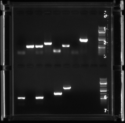
Gel Electrophoresis showing the base pair sizes of dNRG1 PCR
- According to the Fermentes GeneRuler DNA Ladder and the ** list of yeast deletion project primers , placement of the basepairs looks correct. The PCR of DNRG1 was successful.
- Ran the PCR for DPHD1 and made the gel for the gel electrophoresis that I will perform on it Monday morning.
6/10/2015
6/17/2015
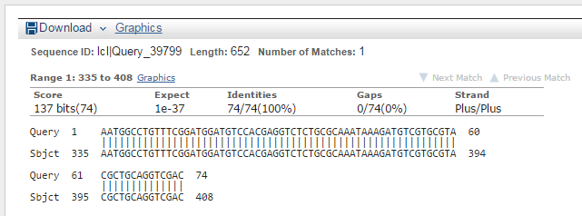
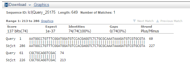
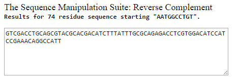
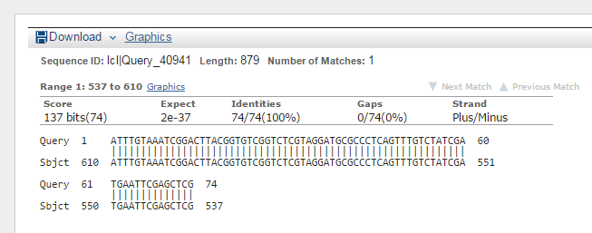
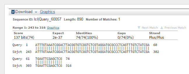
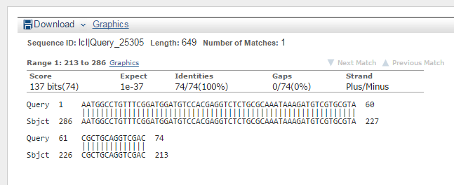
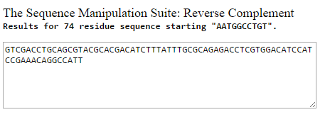
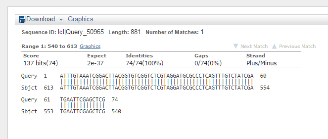
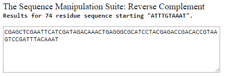
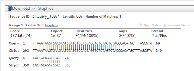
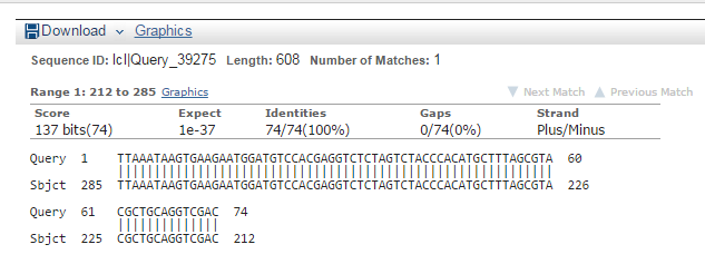
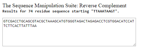
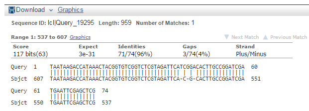
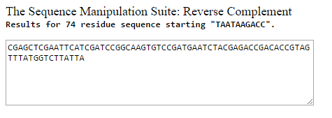
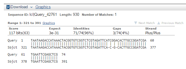
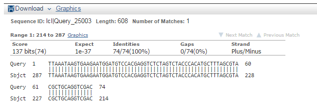
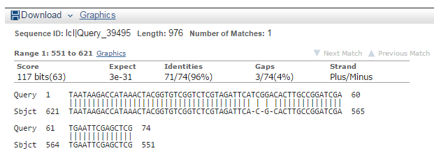
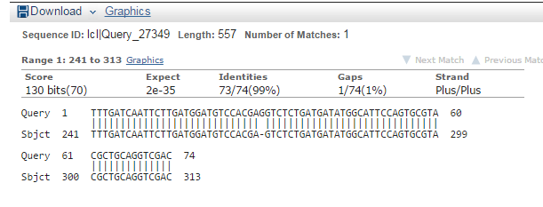
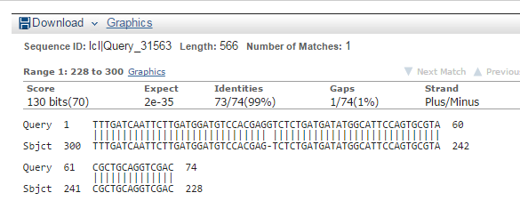
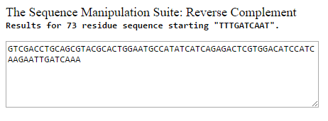
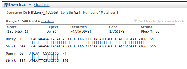
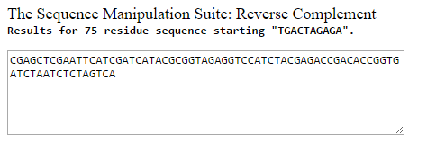
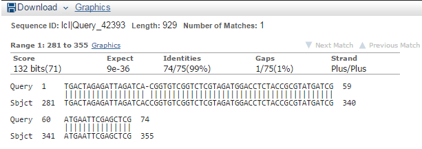
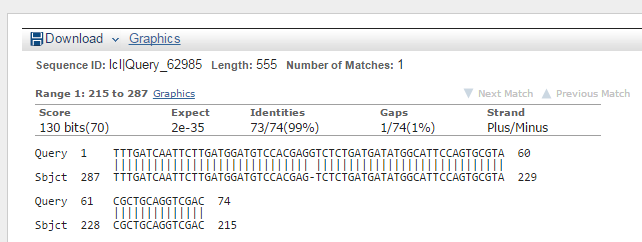
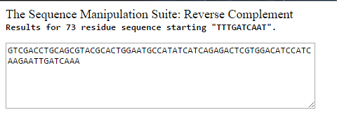
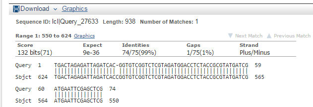
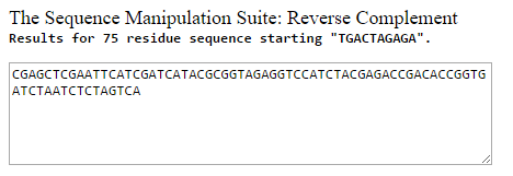
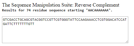
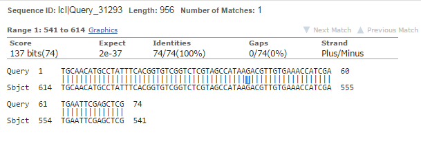
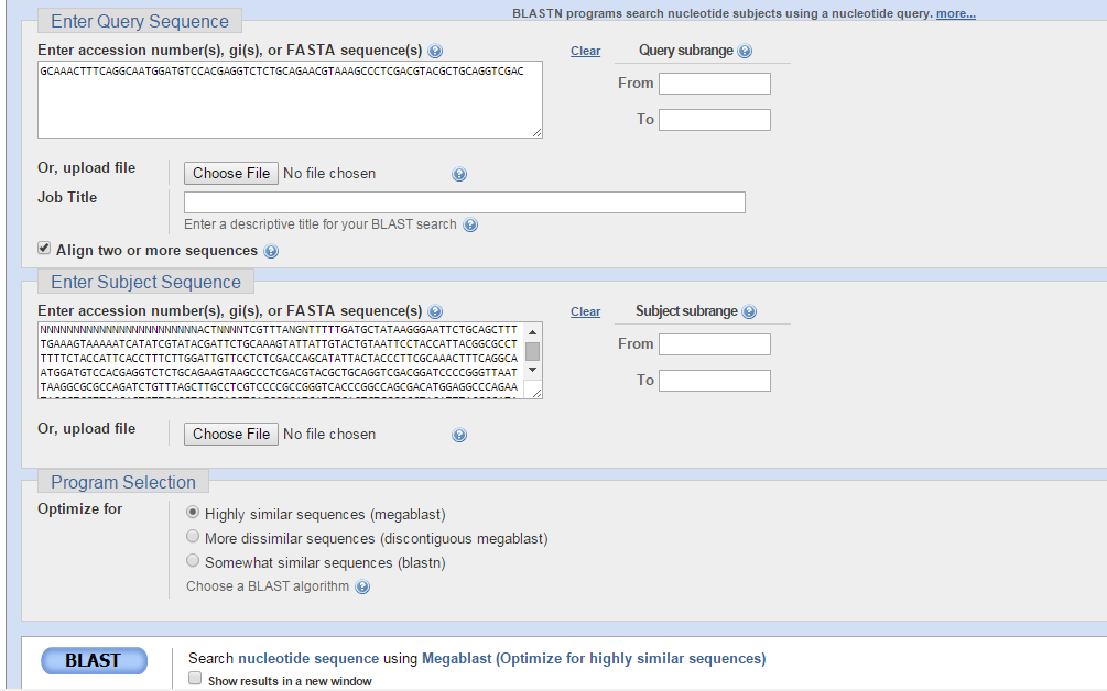
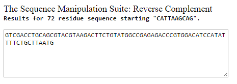
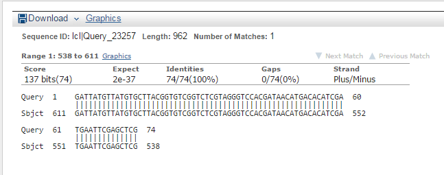
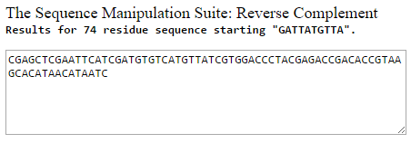
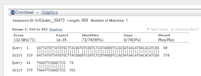
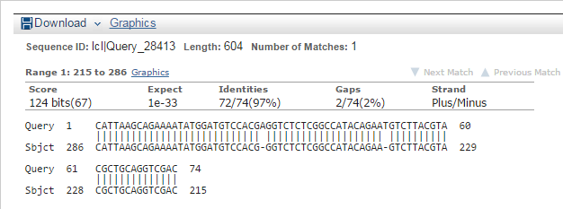
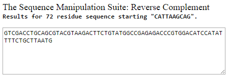
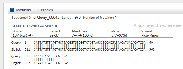
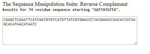
- Used BLAST2SEQ to find the uptag and downtag sequences in the primer sequences
- Here is an example of what the front page should look like:
- I decided that anything with a match to a tag of over 95% should be considered valid. This means that there can be at most 3 errors in between the primer sequence and the tag sequence
- The following are the matches in the primer sequences to the uptag and downtag sequences for NRG1:
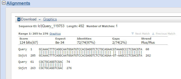
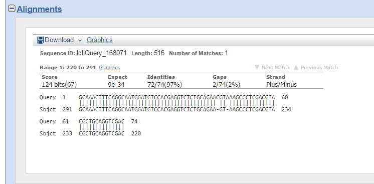
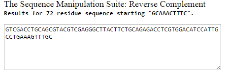
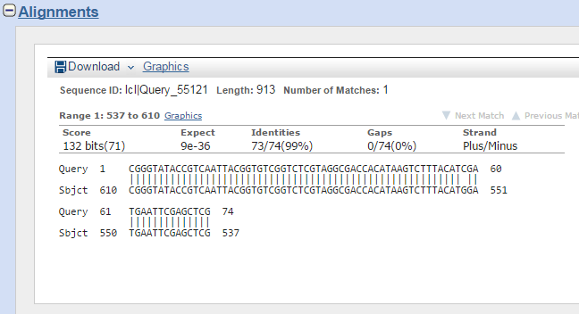
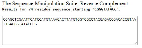
- NRG1 primer D showed an error. I will go back later and troubleshoot the problem
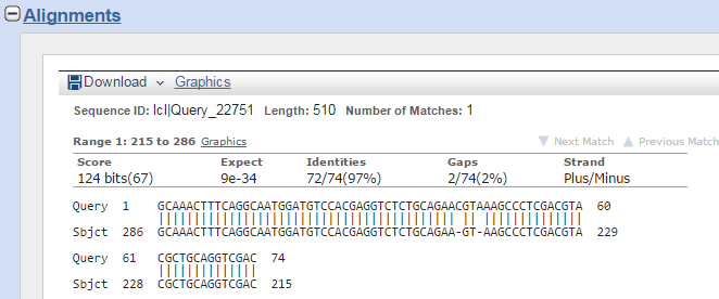
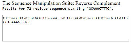

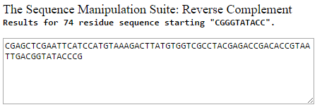
- The Following are the matches in the primer sequences to the uptag and downtag sequences for PHD1:
PHD1 Primer A showed an error. I will go back later and troubleshoot the problem
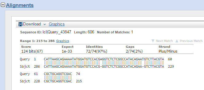
- The Following are the matches in the primer sequences to the uptag and downtag sequences for RSF2:
