Lab 04: Poisson Statistics
Summary
The Poisson Distribution is a discrete probability distribution. It expresses the probability of a number of discrete events occurring within a time frame if the timing of each event is independent of the timing of the previous event and there is a know average rate of events. It is assumed that no two events are simultaneous. If the expected number of occurrences in this interval is [math]\displaystyle{ \lambda }[/math] then the probability that there are exactly k occurrences is equal to
- [math]\displaystyle{ f(k; \lambda)=\frac{\lambda^k e^{-\lambda}}{k!} }[/math]
In the Poisson Distribution, [math]\displaystyle{ \lambda }[/math] is the mean number of occurrences, and [math]\displaystyle{ \sqrt{\lambda} }[/math] is the standard deviation.
In our lab we measured the number of background radiation events in the laboratory. These events should be modeled by a Poisson Distribution because the timing of each of is independent of the timing of the last, the events are highly unlikely to be simultaneous, and it is easy to get a known average of events per dwell time.
We used a scintillator attached to a PMT and wired to a computer to gather the data. When the scintillator absorbs radiation, it fires a beam of ultraviolet light down the tube to the PMT. The PMT then creates a signal voltage that is picked up by a card in the computer. We used the USC 30 software on the computer to set our dwell times and record radiation events. We also used a Spectech Universal Computer Spectrometer power supply to give a bias voltage to the detector. This voltage determines the sensitivity of the detector.
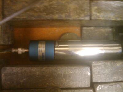
This is the combined PMT scintillator inside 4 short walls of lead bricks
- In this lab I worked with Brian P. Josey.
- These are my Detailed Lab Notes.
Analysis
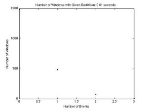
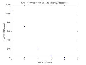
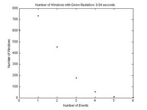
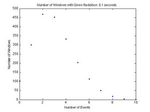
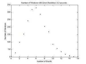
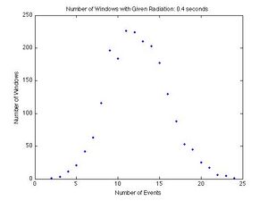
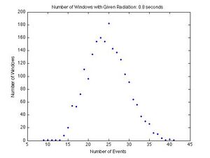
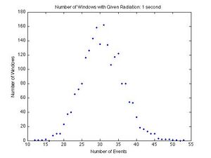
Each graph shows a given number of events for a dwell time on the x-axis, and the number of dwell times in which a given number of events was recorded on the y-axis. If there were 4 dwell times in which 3 events occurred, then 3 is the x-coordinate and 4 is the y-coordinate. Each graph shows the results from a different dwell time. The graphs for the dwell times from left to right and top to bottom are 10, 20, 40, 80, 100, 200, 400, 800 ms and 1 s. As the dwell time increases, the curve becomes symmetric and the peak moves to the right. This is unique of the Poisson Distribution, and a good qualitative test.
To be sure our data represents a Poisson Distribution we compared the standard deviation calculated directly from the data to the root of the mean of the data. The root of the mean of the data is the standard deviation for the Poisson Distribution by definition, so the two numbers should be very close to each other. This is a good quantitative test.
The percent differences are all very small, with the largest being 5.13% and the smallest being 0.18%. This shows that our data does represent a Poisson Distribution reasonably well.
Conclusion
This lab was very easy to do, but it was time consuming. I hadn't studied the Poisson Distribution so the material was new to me. In the future I would recommend that a group do the Poisson Distribution data gathering while working on another experiment since the data gathering takes a few hours and requires very little input from the user.SJK 03:47, 21 December 2010 (EST)

Another idea is that the group could work on creating a LabVIEW or Matlab program to simulate and analyze Poisson data, while waiting for actual data collection.
The results we got from this lab are some of our best in terms of fitting the model we looking for.
